Sector 20 · WCS motion atlas

Focal plane

Scroll to see all four cameras. Each quadrant contains x(t) above y(t). Click a quadrant for larger time series on the right.

Selected position: x above y versus time, with the same vertical scale. The dashed vertical line marks the selected exposure. Coordinates follow the displayed focal-plane axes; units are detector pixels.

x displacement versus time

y displacement versus time

Component	Δx [px]	Δy [px]	Magnitude [px]

Measured lens-barrel temperature

Static figures and the full spatial field

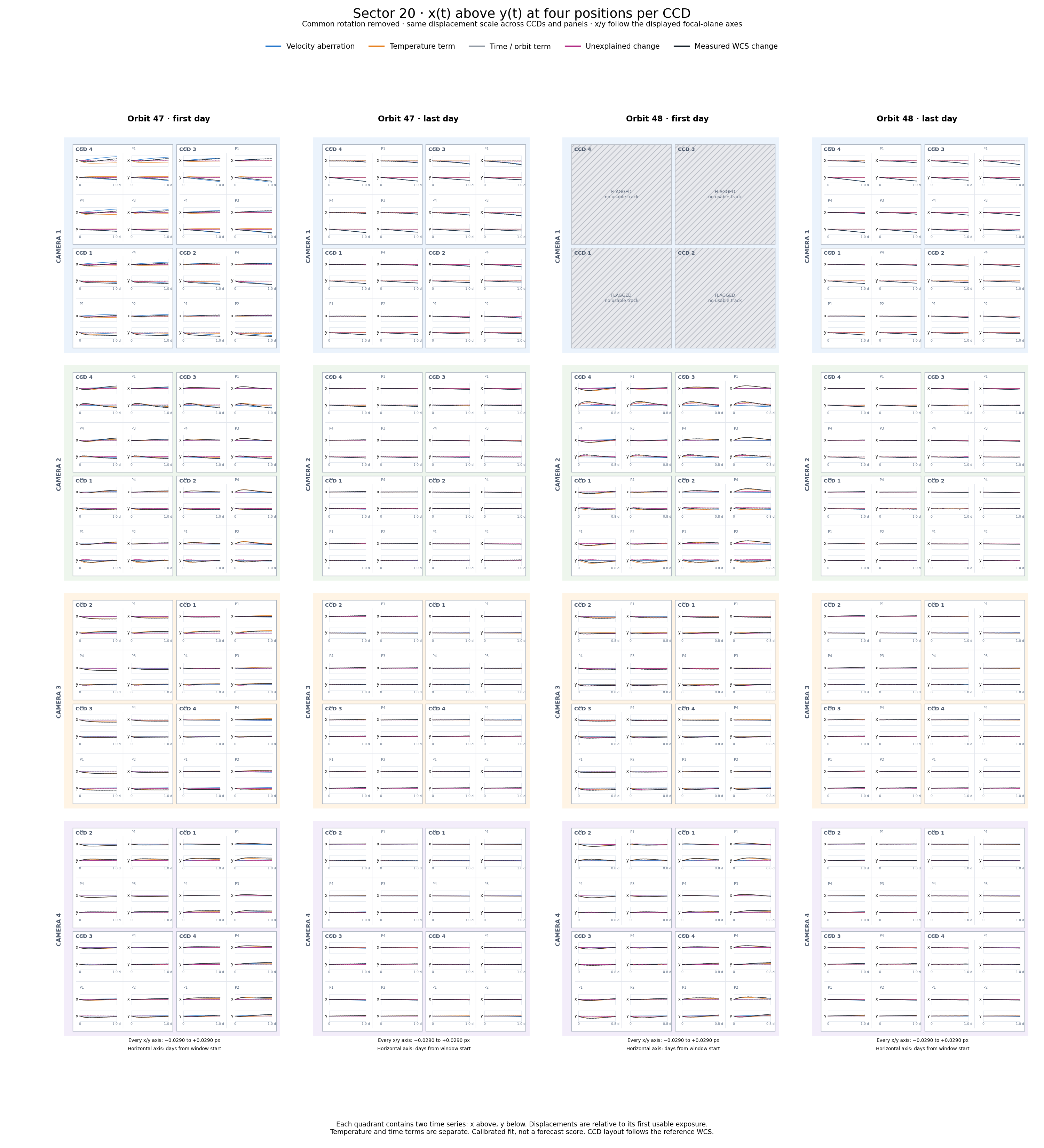
The dense field retains all 81 probes per CCD, rather than only the four representatives. Open a figure for full resolution or use its PDF.

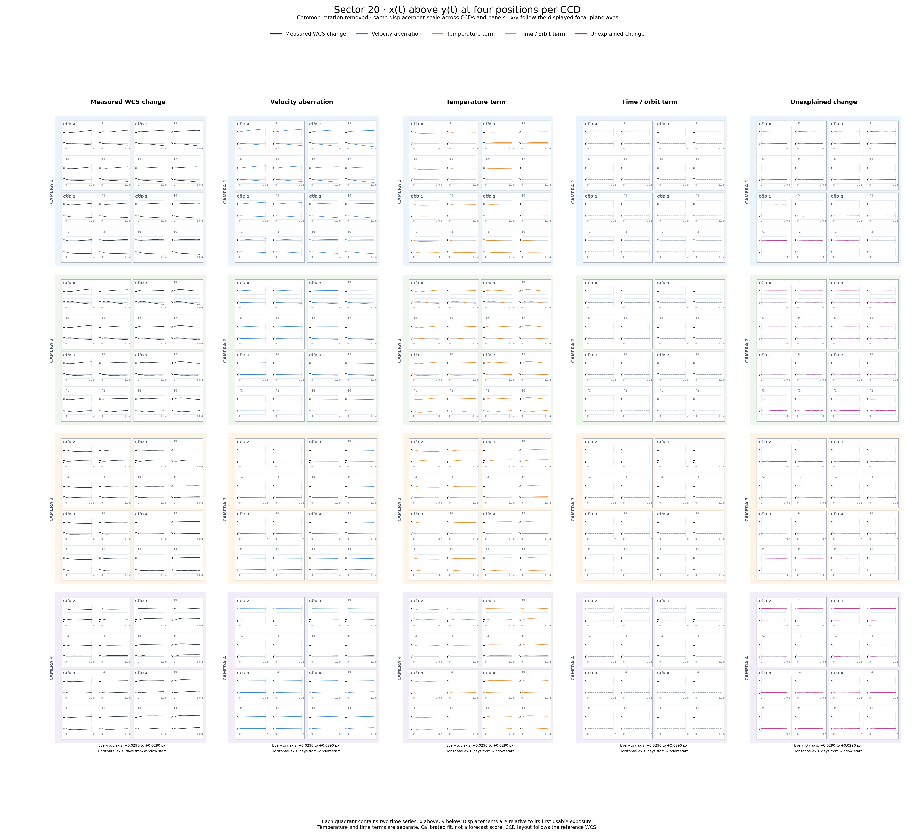
First and last days · PNG Measured VA temperature time and residual fields separately

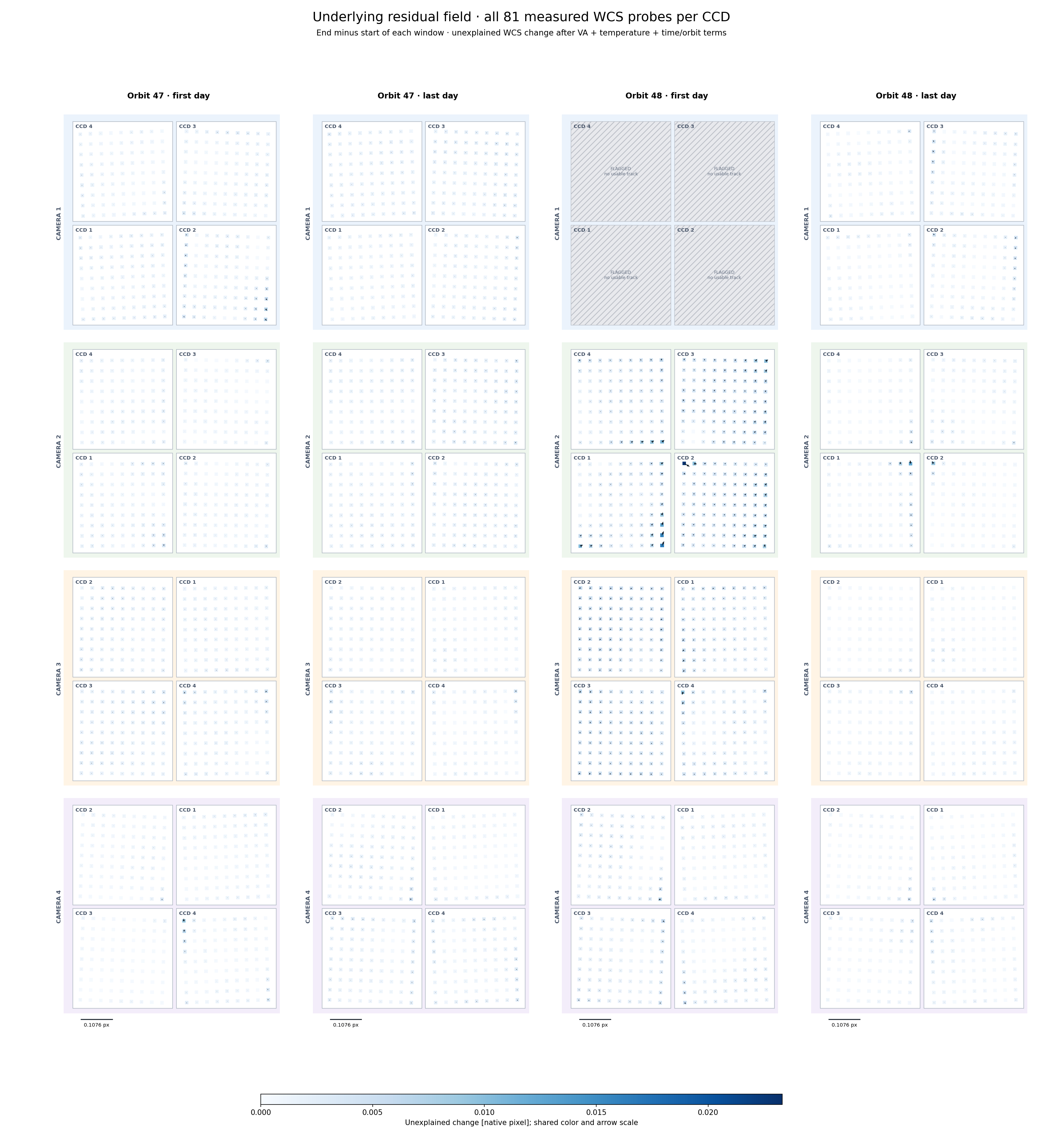
Separate components · PNG Residual vectors at all 81 CCD probes

Underlying residual field · PNG Full orbit 47 motion atlas

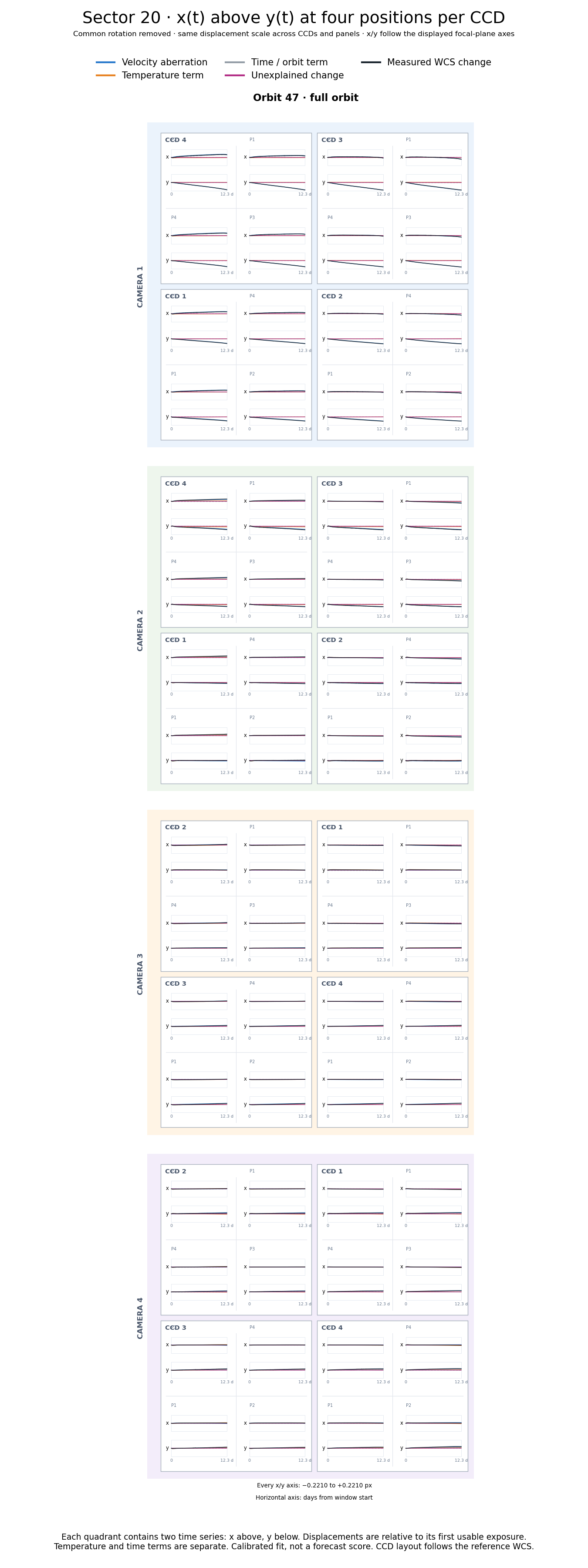
Full orbit 47 · PNG

Endpoint PDF · Component PDF · Residual PDF · Methods and experiment record · Numerical amplitudes

How does the effective “guide star” move in 2D?

These east–north tracks show the reconstructed inertial pointing of a fixed focal-plane ray passing through each orbit’s fitted effective guide center at its middle exposure. The reconstruction uses the measured common WCS attitude and inverse velocity aberration. It is a pointing-drift diagnostic at the guide location, not a direct measurement of an individual star or the onboard ensemble weights.

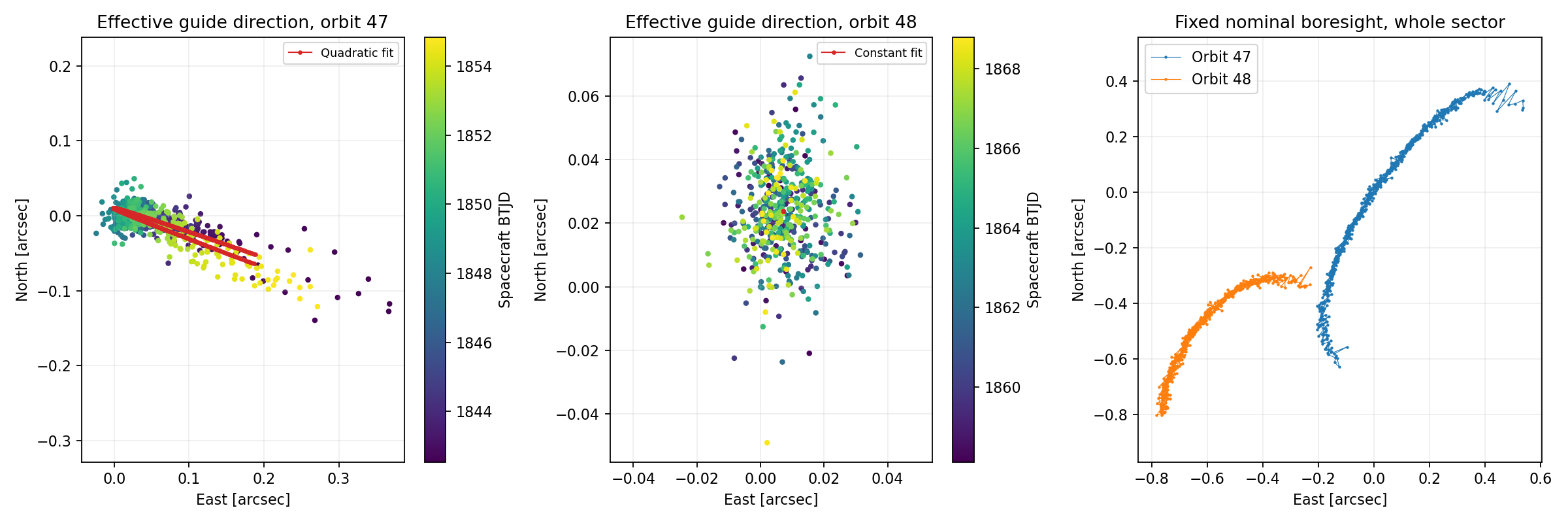
East versus north pointing drift: orbit 47, orbit 48, and the nominal boresight

Reading the plot: horizontal = east, vertical = north, both in arcseconds. Color progresses from purple (earlier) to yellow (later); the color bars give spacecraft BTJD. Each guide panel has its own middle-exposure zero and scale. The red curves are full-data quadratic (orbit 47) and constant (orbit 48) fits. The right panel follows one nominal boresight with a common sector reference; it is a different ray, so its track differs.

Coverage: these are the earlier all-CCD-clean tracks. They exclude the flagged orbit-48 startup; the tight orbit-48 cloud must not be read as evidence that startup was stable. These overview figures show both full orbits and do not change with the atlas time-window controls above.

Pointing drift versus a moving guide-star ensemble

A changing weighted ensemble can move its effective guide location across the sky, while the residual pointing at an adopted guide location is measured on an arcsecond scale. Those are different quantities. Our proxy ensemble fits are model-dependent and do not uniquely identify the true guide-star weights. The plot above displays the reconstructed pointing drift, not the degree-scale fitted migration of that ensemble.

Full-resolution PDF · Per-exposure measurements and fits (CSV)

Conclusion: orbit 47 has a time-dependent pointing drift at its fitted guide location; orbit 48’s clean portion is more stable. This does not establish a unique physical motion of the onboard guide-star average.

MEASUREMENTS, EQUATIONS, AND LIMITS

What each curve means

This atlas decomposes measured WCS-map changes. The velocity is independently supplied by the ephemeris; common pointing/roll is fitted from each exposure; temperature and time coefficients are calibrated against the WCS residuals. The VA response is specified by a physical formula without fitting its amplitude to these WCS changes. A small residual on this page is not a demonstration that velocity and temperature predict the entire WCS.

Curve	Where it comes from	What is estimated
Black · measured	Per-exposure FFI-header WCS, sampled at fixed detector pixels	Data product being explained; not a temperature prediction
Blue · VA	Exact aberration transform using the saved full barycentric spacecraft velocity	No adjustable VA amplitude in this atlas
Teal · common apparent rotation	One three-component rotation fitted independently to each exposure, using cameras 2–4	Measured common pointing/roll; not a recovered guide-star catalogue
Orange · temperature	Fitted spatial response to measured thermistor channels	Regression coefficients and, for camera 2, temperature principal components
Gray · time/orbit	Separate intercept, orbit offset, and per-orbit linear time terms	Empirical baseline coefficients; no thermal mechanism is assigned
Magenta · unexplained	Measured field minus the other terms, in the same coordinate convention	No further fit; may contain real motion, WCS/PSF systematics, noise, and model error

1. Black: how the WCS is measured and sampled

All-CCD data source. For each exposure and CCD, the analysis reads the published WCS in the FFI FITS header, using ffi_list.parquet where available and the actual science-extension FITS header for legacy CCDs. Astropy's WCS(..., relax=True).all_pix2world(..., origin=0) evaluates the map, including the distortion terms in that header. The inspected header examples use TAN-SIP celestial WCS. We do not refit the upstream mission star solution here, and do not infer its original star selection or weights from the header alone.

The matched data contain 1,168 exposures on all 16 CCDs. Each map is evaluated on a 9×9 grid, inset from the science edges: full-FFI x runs from 144 to 1991 pixels and y from 100 to 1947 pixels. The atlas displays four of these actual grid probes per CCD, at the listed quadrant positions. They are fixed detector locations, not four tracked guide stars. The dense residual figure retains all 81 probes.

(\alpha_i(t),\delta_i(t))=W_t(\mathbf p_i),\qquad \mathbf n_i(t)=\begin{bmatrix}\cos\delta_i\cos\alpha_i\\\cos\delta_i\sin\alpha_i\\\sin\delta_i\end{bmatrix}.

$i$ and $t$: Probe index and exposure time; $t$ is spacecraft TDB BTJD, in days.
$\mathbf p_i$: Fixed full-FFI detector coordinate $(x_i,y_i)$ , in zero-based pixels; taken from the stored probe grid.
$W_t$: The exposure's measured header WCS mapping pixels to celestial coordinates.
$\alpha_i,\delta_i$: Right ascension and declination from that map, converted to radians for this expression.
$\mathbf n_i$: Dimensionless three-component unit sky direction; derived from the measured WCS.

To express sky-map changes in detector-pixel units, use the local reference Jacobian:

J_i=\left.\frac{\partial\mathbf n}{\partial(x,y)}\right|_{\mathbf p_i,t_{\rm ref}},\qquad \mathbf m_i(t)=J_i^+\,[\mathbf n_i(t)-\mathbf n_i(t_{\rm ref})].

$t_{\rm ref}$: The common sector reference: cadence tess2019365025923, spacecraft BTJD 1848.63578391. This is distinct from the selected window's display zero.
$J_i$: A 3×2 Jacobian in unit-direction change per native detector pixel. It is computed from the reference WCS by centered finite differences at ±0.01 pixel.
$+$: Moore–Penrose pseudoinverse, converting a small sky-vector change into two pixel components.
$\mathbf m_i$: The measured two-component WCS-map displacement, in native pixel units. Its total-motion version is the black curve before display rotation/recentering.

This is a local linear conversion of an evaluated celestial map, not a direct inverse-WCS remeasurement of a star's detector position. A fixed star's centroid movement has approximately the opposite sign at first order. Static WCS offsets cancel in the reference difference; shared or time-dependent errors in the original WCS can remain.

What the TAN-SIP header map contains

For TAN-SIP headers, the conceptual pixel-to-sky mapping is

u=x+1-\mathrm{CRPIX1},\quad v=y+1-\mathrm{CRPIX2},\qquad F_A(u,v)=\sum_{r+s\ge2}A_{rs}u^rv^s,\quad F_B(u,v)=\sum_{r+s\ge2}B_{rs}u^rv^s.

$x,y$ and $u,v$: Zero-based full-FFI coordinates and offsets from the FITS reference pixel, all in pixels. The +1 converts the analysis's zero-based coordinates to the header's one-based CRPIX convention; Astropy handles this conversion.
CRPIX1, CRPIX2: Reference-pixel coordinates supplied in that exposure's FITS header, in one-based pixels.
$r,s$ and $A_{rs},B_{rs}$: Nonnegative polynomial powers and the corresponding forward SIP distortion coefficients from the header. The sums include only the terms present through the header's specified orders. A coefficient multiplying a degree- $r+s$ term has units of pixels to the power $1-r-s$ .
$F_A,F_B$: The two polynomial distortion offsets, in pixels; these are header coefficients, not the orange temperature fit.

\begin{bmatrix}\xi\\\eta\end{bmatrix} =M\begin{bmatrix}u+F_A(u,v)\\v+F_B(u,v)\end{bmatrix},\qquad (\alpha,\delta)=\operatorname{TAN}^{-1}_{(\mathrm{CRVAL1},\mathrm{CRVAL2})}(\xi,\eta).

$M$: The header's linear WCS transform, represented by CD or by PC plus CDELT, in angular units per pixel.
$\xi,\eta$: Tangent-plane coordinates in the header's angular units; here the celestial WCS uses degrees.
CRVAL1, CRVAL2 and TAN inverse: The header's reference sky coordinate and inverse gnomonic projection. They convert tangent-plane positions into the right ascension/declination already defined above.

This explains the map being evaluated, not the upstream mission procedure that fitted its coefficients. The atlas reads those coefficients as supplied. A time-dependent header coefficient can represent pointing, optical distortion, or an upstream fitting error; its physical interpretation is what the subsequent decomposition tests.

Independent centroid-derived check. C3/CCD3 also has existing centroids_r1 measurements and per-exposure degree-5 Chebyshev WCS fits under wcs/per_ffi_cheb5. That model maps the Gaia tangent-plane coordinates to detector coordinates. For the independent analysis, the saved coefficients from each exposure replace the temporal store's coefficients, so the plotted comparison in the earlier investigation uses the unsmoothed per-exposure solution. Its science-local origin is offset by (44, 0) full-FFI pixels. Those centroid-derived maps do not supply all 16 black curves on this webpage. The original per-exposure fitter's star selection/weights are not reconstructed by this visualization; shared ePSF biases are still possible.

Timing and flags. Spacecraft midpoint is computed from each header as follows; the global comparison uses the mean of the staggered CCD times.

t=\tfrac12(\mathrm{TSTART}+\mathrm{TSTOP})-\mathrm{BARYCORR}.

TSTART and TSTOP: Header exposure endpoints, in the TESS day-based time convention.
BARYCORR: The header barycentric light-time correction, in days, removed to obtain spacecraft time for the ephemeris.

A CCD's displayed track uses only exposures with its DQUALITY=0. Camera 1 has no usable first-day orbit-48 track; cameras 2–4 do. The calibration used the stricter 1,100-exposure sample clean on every CCD. Thus displaying unflagged startup measurements from cameras 2–4 does not mean those exposures trained the orange model.

2. Blue: velocity aberration from the full spacecraft velocity

The saved lkspacecraft/SPICE state vectors use definitive TESS ephemerides, DE440s, and the leap-second kernel. The barycentric velocity includes both Earth's motion and TESS's motion relative to Earth; the varying near-Earth orbital speed is included. The source-direction transform is

A(\mathbf n,\boldsymbol\beta)= \frac{\mathbf n/\gamma+\boldsymbol\beta+ \frac{\gamma}{\gamma+1}(\boldsymbol\beta\cdot\mathbf n)\boldsymbol\beta} {1+\boldsymbol\beta\cdot\mathbf n},\qquad \boldsymbol\beta=\frac{\mathbf u}{c},\qquad \gamma=(1-\lVert\boldsymbol\beta\rVert^2)^{-1/2}.

$A$: Exact special-relativistic aberration transform used by the analysis; its output is an observer-frame unit source direction.
$\mathbf n$: A unit celestial direction evaluated from the WCS, as defined above.
$\mathbf u$ and $c$: Independently supplied full barycentric spacecraft velocity in km/s, and the constant speed of light, 299,792.458 km/s.
$\boldsymbol\beta$ and $\gamma$: Dimensionless velocity and Lorentz factor, calculated from the ephemeris, not fitted to the curves.

Apply the transform to the measured WCS directions and form the apparent-frame change:

\mathbf a_i(t)=A(\mathbf n_i(t),\boldsymbol\beta_t),\qquad \mathbf o_i(t)=J_i^+\,[\mathbf a_i(t)-\mathbf a_i(t_{\rm ref})],\qquad \mathbf v_i(t)=\mathbf m_i(t)-\mathbf o_i(t).

$\mathbf a_i$: Dimensionless apparent direction after applying aberration to the measured celestial direction.
$\mathbf o_i$: Apparent-frame WCS change in pixel units, using the same reference Jacobian.
$\mathbf v_i$: The full VA contribution in pixel units, defined by the difference between the celestial and apparent changes. This is the blue term in total-motion mode, before display recentering.

The transform is evaluated on the measured rays to give a consistent decomposition; this blue term is not a free-amplitude fit or a guide-star fit. The amplitude is fixed at one. In distortion mode, the same common-rotation-removal operator acts on this term, leaving its differential spatial component. The page uses midpoint velocity; the separate exposure-integration check in the investigation found only a very small correction.

3. Teal: common apparent rotation — measured pointing and roll

This term is fitted independently for every exposure. It is the best-fit three-dimensional rotation that moves the apparent directions together. It describes a shared pointing/roll change, not a physical rotation of each CCD. “Apparent” refers to the observer-frame directions after applying aberration.

D_i\boldsymbol\omega=J_i^+\,[\boldsymbol\omega\times\mathbf a_i(t_{\rm ref})],\qquad \widehat{\boldsymbol\omega}(t)=(SD)^+S\mathbf o(t),\qquad \mathbf p(t)=D\widehat{\boldsymbol\omega}(t).

$\boldsymbol\omega$ and $\widehat{\boldsymbol\omega}$: A small three-component rotation vector, in radians, and its fitted value for the exposure. Its components encode common pointing and roll.
$D_i$ and $D$: The probe's 2×3 rotation design matrix, in pixels per radian, and the matrix formed by stacking all probe rows. The cross product specifies its sign convention.
$S$: A dimensionless row-selection matrix retaining all 81 probes on each of the twelve CCDs in cameras 2–4.
$\mathbf o$: The concatenated apparent-frame changes over all 16 CCDs, in pixels.
$\mathbf p$: The fitted common apparent rotation evaluated at every probe, in pixels; the teal total-motion curve.

The pseudoinverse gives an unweighted least-squares fit to those probe components. The 81 probes on a CCD are samples of a WCS model, not 81 statistically independent stars. Camera 1 is excluded from the rotation estimate throughout both orbits so its contaminated epochs do not enter indirectly.

Q=I-D(SD)^+S,\qquad Q\mathbf o=\mathbf o-\mathbf p.

$I$ and $Q$: The identity matrix on the full stacked field and the dimensionless common-rotation-removal operator. The same $Q$ acts on all components; it is defined by the twelve-CCD fit, not an independent per-CCD recentering.

The default black curve is based on $Q\mathbf m$ , and the default blue curve on $Q\mathbf v$ . Both have their common rotational component removed. This is more precise than saying that only the teal curve was subtracted from the black one: the common VA component is projected out too. Full-motion mode restores the unprojected black/blue terms and shows the teal contribution explicitly.

Because this fit uses the measured WCS, it can absorb real attitude motion, guiding compensation, and optical changes that resemble a common rotation. It is not a unique measurement of the onboard guide-star average, and is not the VA-plus-guide-center forecast tested elsewhere. Scale changes, shear, and differential camera/CCD motion are not fully represented by a single common rotation.

4. Orange: temperature-associated spatial distortion

Temperature comes from the downloaded sector-20 engineering FITS file found with tess_sector20_telemetry.ipynb. Nine pt1000 channels per camera are available: hood (1), barrel (2–5), FPE housing (6–7), FPA housing (9), and FPA mosaic (10). Samples are cleaned for invalid values and isolated spikes and averaged over each 30-minute exposure, with at least ten telemetry samples required. The orange curve uses the instantaneous exposure-averaged model, not a delayed thermal state.

Camera	Saved temperature features	Ridge penalty
1	Six physical channels: mean barrel, hood, mosaic, FPA housing, mean FPE housing, barrel gradient (sensor 2 minus 5)	10
2	First three principal components of all nine standardized thermistors	1
3	The same six physical channels as camera 1	1
4	All nine thermistors	1

Feature representation and ridge penalty were selected with buffered time folds. The displayed archive then refits the selected model on all 1,100 all-CCD-clean exposures. Normalization and PCA are stored with that calibration. The lens-barrel line below the selected-position plots is one sensor for context; it is not the entire orange predictor.

Each CCD's spatial field is compressed into an orthonormal basis spanning total-degree-5 polynomials on its 81 probes. There are 21 spatial basis functions for each of the two displacement coordinates. Temperature and time predictors fit the temporal coefficients:

\mathbf f_{ij}(t)=\sum_{k=1}^{21}\phi_{jk}(\mathbf p_i)\sum_{\ell=1}^{L_j}X_{j\ell}(t)\,\mathbf C_{jk\ell}.

$j$: CCD index, with the temperature predictors selected for its parent camera.
$\mathbf f_{ij}$: The fitted two-component residual field at probe $i$ on CCD $j$ , in pixels, before the atlas's twelve-CCD reprojection.
$\phi_{jk}$: Dimensionless orthonormal spatial basis functions, obtained by QR decomposition of normalized detector monomials through total degree five.
$X_{j\ell}$ and $L_j$: A dimensionless standardized temporal predictor and the number of such predictors. The first four columns are baseline terms; the rest are temperature features.
$\mathbf C_{jk\ell}$: Two-component fitted coefficients in pixels. They are calibrated from WCS residuals, not obtained from a mechanical thermal-expansion model.

In matrix notation, the fitted coefficients solve

\widehat C=\operatorname*{arg\,min}_{C}\left[\lVert Y-XC\rVert_F^2+\lambda\lVert P^{1/2}C\rVert_F^2\right],\qquad P=\operatorname{diag}(0,0,1,\ldots,1).

$Y$: The camera's spatial coefficients extracted from the observed, VA-corrected field after the original all-16-CCD attitude fit; in pixel units.
$X$ , $C$ , and $\widehat C$: The training predictor matrix, coefficient matrix, and its fitted value; these collect the predictors and coefficients in the preceding equation.
$\lVert\cdot\rVert_F$: Frobenius norm, summing squares over training exposures and fitted spatial-coordinate coefficients.
$\lambda$ and $P$: The chosen dimensionless ridge strength and penalty matrix. Intercept and orbit offset are unpenalized; time and temperature predictors are penalized. The implementation adds a $10^{-12}I$ numerical stabilizer to the normal matrix.

The original residual calibration used an all-16-CCD attitude convention on clean exposures. This atlas consistently reprojects its predictions to the twelve-CCD convention; it does not silently refit a different model in the browser.

\mathbf f_T(t)=\text{the part of }\mathbf f(t)\text{ from predictor columns }5\ldots L_j,\qquad \mathbf h(t)=Q\mathbf f_T(t).

$\mathbf f$ and $\mathbf f_T$: The concatenated fitted spatial field and its temperature-column contribution, in pixels. Column numbers here are one-based; the implementation zeroes coefficient rows 0–3 to isolate temperature.
$\mathbf h$: The reprojected temperature-associated field in pixels, giving the orange curve after display recentering.

A successful orange curve shows an empirical relation to temperature in this calibration. Temperature, time, velocity, and orbit phase can be correlated; their fitted coefficients and apparent attribution depend on model specification and regularization. The page does not identify a unique causal thermal fraction. Tested lag/rate models and startup exponential fits belong to the separate endpoint investigation and are not added to this orange term.

5. Gray: time trend and orbit offsets, kept separate from temperature

X_B(t)=\left[1,\ \widetilde o(t),\ \widetilde{\tau(t)\,\mathbb 1_{o=0}},\ \widetilde{\tau(t)\,\mathbb 1_{o=1}}\right],\qquad \mathbf b(t)=Q\,[\mathbf f(t)-\mathbf f_T(t)].

$X_B$: The first four temporal-design columns: intercept, orbit offset, and a separate linear time slope in each orbit.
$o$: The orbit indicator, 0 for orbit 47 and 1 for orbit 48; determined from the observing gap.
$\tau$: Time minus the mean training time, initially in days.
$\mathbb 1$ and the tilde: An indicator equal to one when its condition holds, and centering/scaling by the saved training statistics; the resulting design columns are dimensionless.
$\mathbf b$: The baseline contribution, in pixels, giving the gray curve. The fitted field $\mathbf f$ , its temperature part $\mathbf f_T$ , and the projection $Q$ are defined above.

This term can absorb slow trends and an inter-orbit offset. It is not labeled thermal. Within one orbit, window differencing removes a constant intercept/orbit offset, but a time slope remains. Separating the gray and orange columns prevents the entire regression improvement from being called a temperature effect.

6. Magenta: what remains unexplained

\mathbf r(t)=Q\,[\mathbf o(t)-\mathbf f(t)].

$\mathbf r$: The unmodeled residual field, in pixels. It compares the observed apparent-frame change $\mathbf o$ with the fitted temperature-plus-baseline field $\mathbf f$ after the common-rotation projection $Q$ .

Nothing further is fitted to the magenta term. It can contain optical changes outside the spatial/temporal model, pointing-like motion not captured by the common fit, measurement error, and shared centroid/ePSF systematics. The finite spatial-basis approximation also remains here.

What the page displays is the change in this residual since the selected window's first usable exposure. A constant prediction offset over that window cancels. A small magenta curve therefore cannot be read as a small absolute WCS error, nor as a withheld prediction score. Use the separately reported held-out first/last-day tests for that question.

7. Exact component sums, the two viewing modes, and the plotted x/y axes

\underbrace{\mathbf m}_{\text{total measured}} =\underbrace{\mathbf v}_{\text{VA}}+\underbrace{\mathbf p}_{\text{common rotation}} +\underbrace{\mathbf h}_{\text{temperature}}+\underbrace{\mathbf b}_{\text{time/orbit}}+\underbrace{\mathbf r}_{\text{unexplained}},

\underbrace{Q\mathbf m}_{\text{distortion view}} =Q\mathbf v+\mathbf h+\mathbf b+\mathbf r.

All vectors and the operator in these equations are defined in the sections above and use the same pixel units and reference. The first line describes total-motion mode, including teal. The second describes the default distortion mode. The stored arrays satisfy these identities to floating-point precision; the webpage rounds vector components to six decimals for storage.

Finally, every curve shown in a CCD quadrant is

\mathbf z_i(t)=R_j\,[\mathbf c_i(t)-\mathbf c_i(t_{0,j})],\qquad x_{\rm plot}=z_{i,1},\quad y_{\rm plot}=z_{i,2}.

$\mathbf c_i$: Whichever measured/model component is being displayed, in the selected total-motion or distortion convention.
$t_{0,j}$: The first usable exposure of CCD $j$ within the selected window. It can be later for camera 1 in a full-orbit window; the detail panel states the zero epoch.
$R_j$: A fixed dimensionless orthogonal transformation derived from the reference WCS, orienting native detector vectors into the displayed focal-plane axes. It preserves lengths and can reverse the local detector axes on differently oriented CCDs.
$\mathbf z_i$ , $x_{\rm plot}$ , and $y_{\rm plot}$: The window-relative displayed vector and its horizontal/vertical components, in native-pixel units. They follow the focal-plane display orientation, not necessarily the raw column/row signs of that CCD.

The two plots inside each quadrant show $x_{\rm plot}(t)$ above $y_{\rm plot}(t)$ . All mosaic panels share a displacement scale and the selected time range. The horizontal axis is elapsed days since the window's first sampled time. Magnification can clip curves; the page warns when it is enabled. Playback steps through observed cadences, including the actual time gaps.

Components add as signed vectors, not as positive amplitudes or percentages. Large VA and common-rotation terms can cancel in total-motion mode. No new physical information is created by this algebraic closure.

8. What is validated, what remains conditional, and where the inputs live

The camera representation and penalty choices were tested with buffered time folds. The preceding endpoint study used whole first/last-day holdouts, and the broader analysis used five contiguous outer blocks per orbit with a 0.25-day exclusion buffer and training-only inner selection. This page displays the final full-data calibration, not those cross-validation predictions. Common rotation is always inferred from the measured WCS of the exposure being displayed.

All-CCD black curves: header WCS evaluated on fixed probes; no independent remeasurement of all stars is performed by this page.
Independent unsmoothed centroid WCS: C3/CCD3 only. Shared ePSF error is not excluded by that comparison.
VA: supplied full velocity, exact aberration expression, unit amplitude. The decomposition evaluates it at the measured rays.
Teal: measured from each exposure, with 3 rotation parameters; it does not predict the initial pointing transient.
Orange/gray: calibrated coefficients. Flagged camera-1 data are excluded; unflagged camera-2–4 startup displayed here includes times excluded from the all-CCD-clean training sample.
Magenta: window-relative remaining change, not absolute forecast accuracy or photometric precision.

Input records available through this same server: WCS/telemetry inventory, engineering and ephemeris provenance, selected thermal calibration, withheld distortion scores, twelve-CCD startup scores, atlas manifest, and browser and vector-closure checks.

Representative source locations are /astro/armin/koji/syndiff/data/s0020/c*/k*/ for the FFIs and header records; /astro/armin/koji/syndiff/data/s0020/c3/k3/wcs/per_ffi_cheb5/ for the independent centroid solution; and the engineering downloads alongside /home/kshukawa/syndiff_pipeline/dev/pointing_analysis/tess_sector20_telemetry.ipynb. Cached analysis inputs are in this run's baseline_results/. The webpage reads those saved results; changing its controls does not refit the WCS or temperatures.

Conclusion: the atlas is a consistent decomposition of measured WCS changes into a prescribed VA correction, a measured common rotation, fitted temperature/time responses, and remaining change. It shows where the calibration follows the data, while leaving the initial-pointing prediction, unique thermal causation, and end-to-end light-curve accuracy as separate tests.