Does bad nonlinearity calibration flatten the peaks?
A response-like component is present, but these tests do not identify a bad nonlinearity correction as the common cause. The intended correction is applied accurately in the tested pixels. A diagnostic correction removes part of the bright-star pattern; substantial structure remains, and broadening can explain part of the same signal.
2026-10-02 · SynDiff investigation · No production calibration or science image changed.
1. Verify the operation before changing the detector model
Five raw/calibrated FFI pairs span S24 C2 K2 (four epochs) and S20 C3 K3 (the exact morphology-test epoch). We reverse the candidate archival flat, subtract the static bias map, estimate the remaining row bias from trailing collateral pixels, and project out additive row/column effects. A cubic response is fitted on one checkerboard half and checked on the other. The nuisance row/column projection on evaluation pixels is conditional; this is a transfer-reconstruction test, not an independent detector calibration.
The measured response agrees with the independently maintained TICA implementation's transformed SPOC coefficients. The raw archival XML coefficients are not a direct multiplicative response: that interpretation produces a false discrepancy. The small remaining nearly linear difference is at sub-ppm relative gain scale; rounded coefficients and exposure normalization limit this reconstruction. This rules against an omitted, doubled or grossly mis-scaled application in these images. It does not establish that the laboratory response is still physically correct.
Definitions
$$u_{p}=R_p/N-B_p-b_{r(p)},qquad v_p=C_p F_p E/(Ng_{a(p)}).$$
Here (p) labels a pixel; (R_p) is the archived raw coadd in ADU; (N) is the header's retained-read count (720 for the tested 30-minute FFIs); (B_p) is the candidate static bias map in ADU/read; (b_{r(p)}) is the row-dependent bias estimated from trailing collateral pixels, also ADU/read; (C_p) is the calibrated pixel rate in electrons/second; (F_p) is the dimensionless archival flat; (E) is header exposure in seconds; and (g_{a(p)}) is the header gain in electrons/ADU for output (a(p)). Thus (u_p) and (v_p) are both mean ADU/read. Additive row/column terms absorb remaining bias/smear in the comparison.
$$v_psimeq u_p,[a+b,s(u_p-o)+c,s^2(u_p-o)^2].$$
The dimensionless (a,b,c), scale (s) in inverse ADU, and origin (o) in ADU are the fixed transformed SPOC response parameters from pinned TICA source. Their accuracy as applied coefficients is tested here; they are not fitted to stellar shapes.
Across 20 output/epoch fits, the largest relative difference in the fitted quadratic/cubic coefficients is 10.7 ppm of the coefficient itself. This is not a bound on absolute detector calibration error.
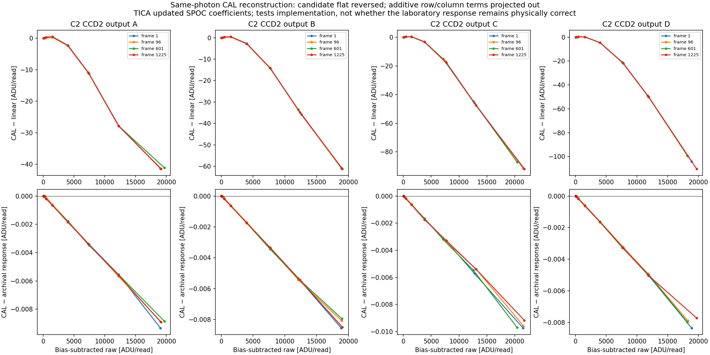 S24 C2 K2: actual CAL-minus-linear transfer (top) and residual against transformed SPOC response (bottom). The bottom scale is thousands of times smaller.
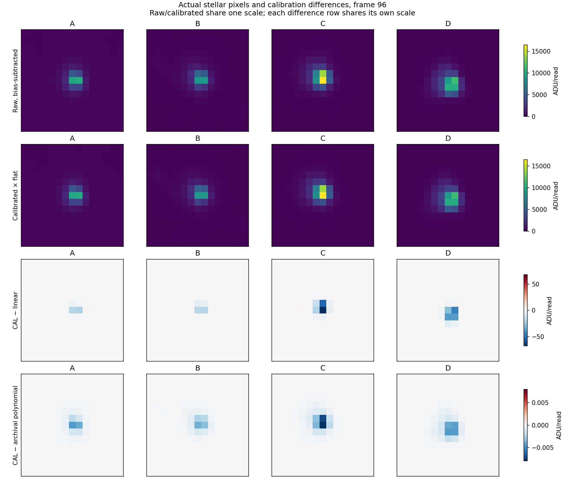 Underlying unsaturated stellar pixels for the same test. First two rows share a scale; each difference row has its own shared scale.
Independent C3 K3 reconstruction and alternative response family
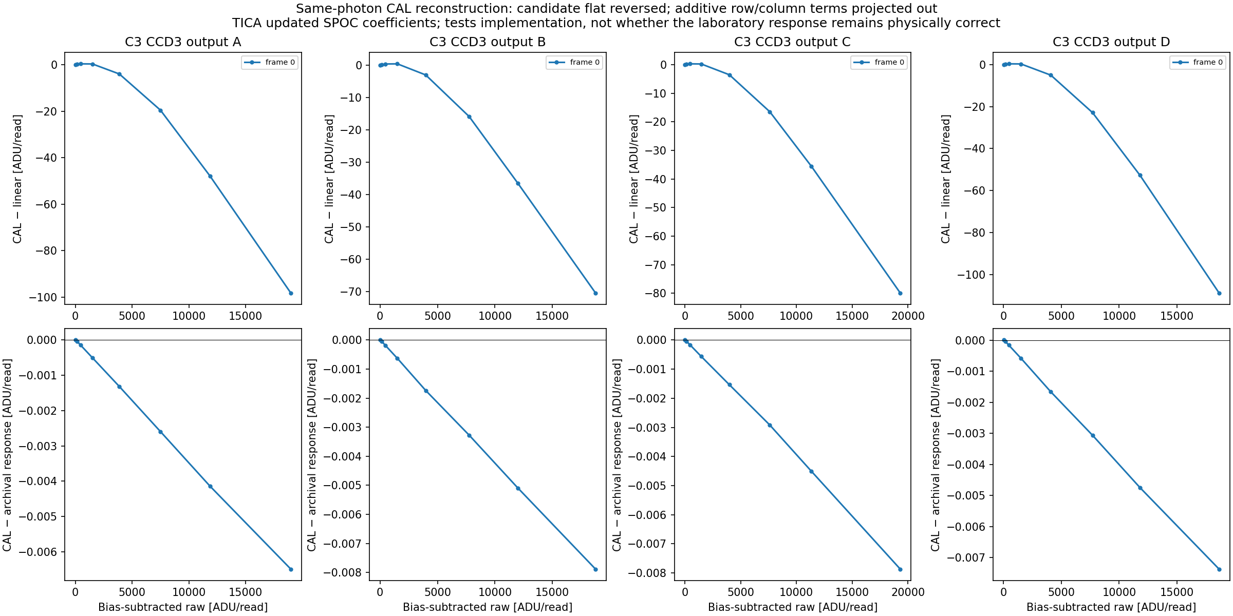 S20 C3 K3, exact epoch used in the calibrated-FFI morphology test.
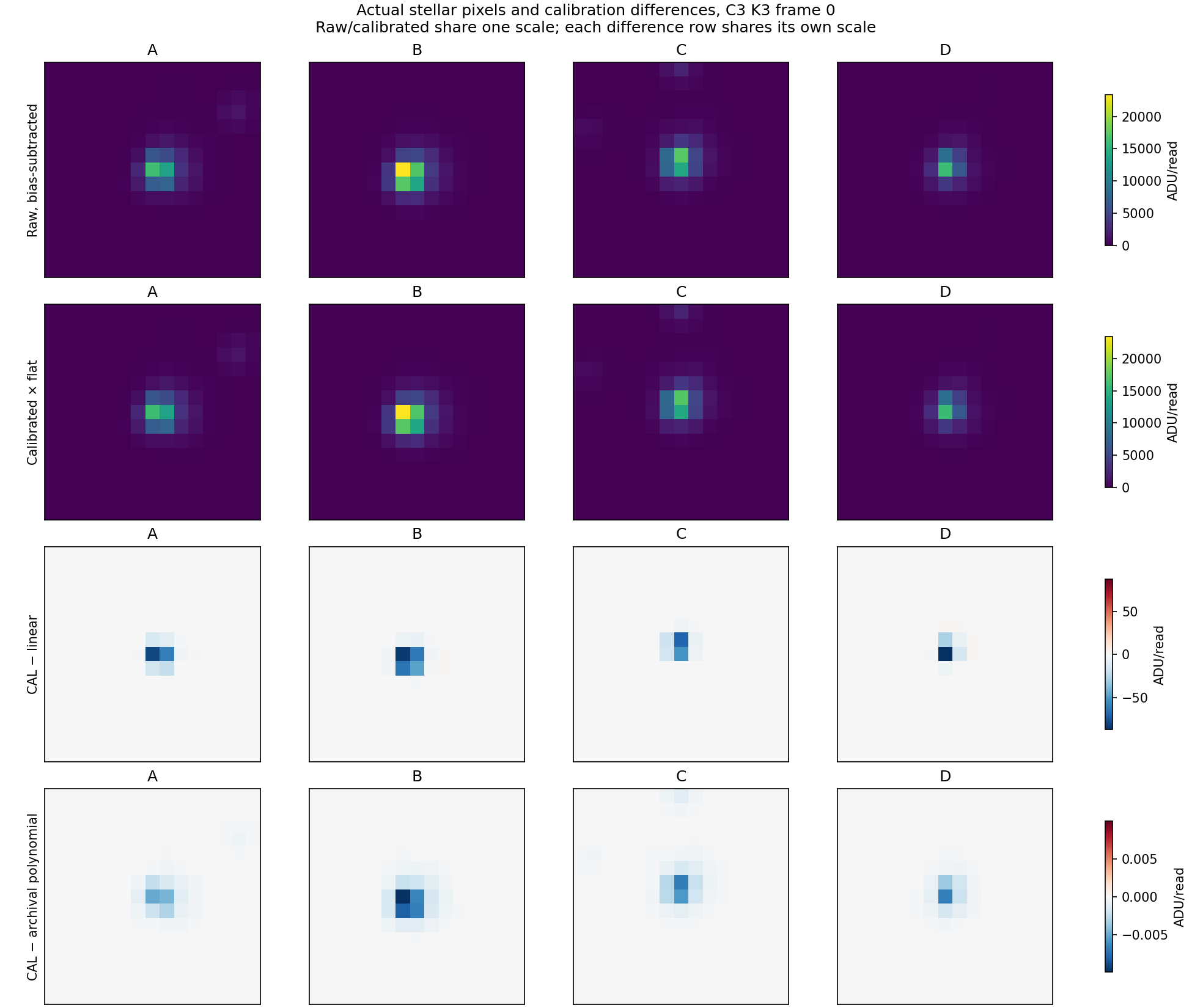 The actual C3 K3 pixels underlying the reconstruction.
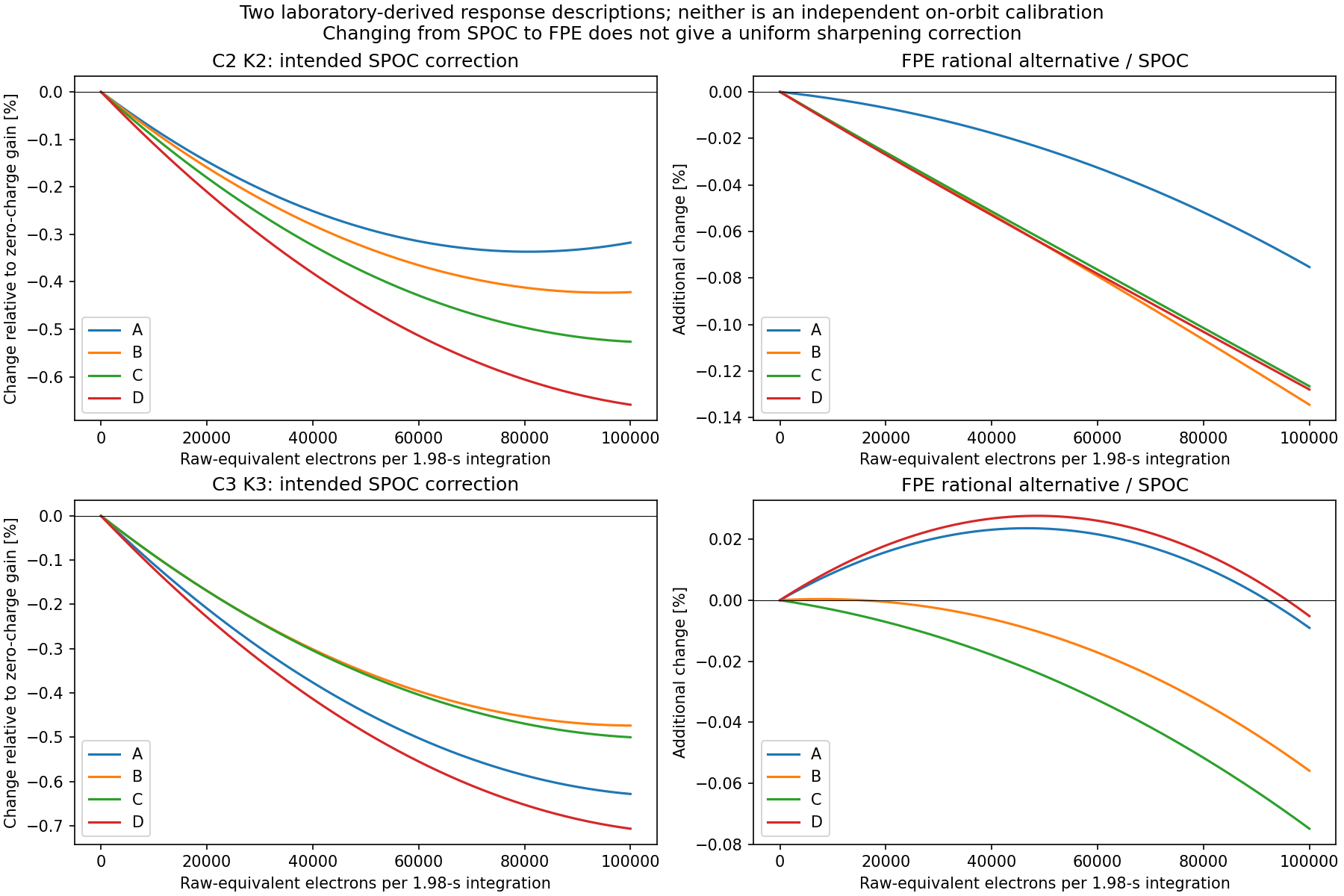 The handbook/FPE rational response and intended SPOC response are related laboratory descriptions, not independent on-orbit truth. Their difference is channel dependent and is not a uniform sharpening fix.
2. Test a candidate correction against competing shapes
We test a small quadratic detector-response residual:
$$q'_{ip}=q_{ip}+kappa_a q_{ip}^{,2},qquad q_{ip}=t_{
m int}f_iP_{ip}.$$
Here (i) labels a source and (p) a pixel; (q_{ip}) and (q'_{ip}) are raw-equivalent charges in electrons per integration before/after a hypothetical residual response; (t_{
m int}=1.98) seconds is the header integration time; (f_i) is the saved fitted flux in electrons/second; (P_{ip}) is that source's saved normalized pixel model; and (kappa_a), in inverse electrons, is a fitted coefficient shared by readout output (a). Negative (kappa_a) suppresses the peak. This approximation is conditional on the saved model and is not an absolute charge calibration. For hp_d, removed scene light is absent, so fitted coefficients cannot directly be applied to raw detector pixels.
Its normalized residual template is (t_{
m int} f_i P_{ip}^{,2}). We compete it with second spatial derivatives of the local model, allowing independent row, column and cross-width terms. Flux, centroid shifts and a local sky plane are projected out on fixed pixels. The baseline already fits local shape dependence on position and Gaia BP−RP colour (including colour squared); it has no brightness term. The compared additions are response alone, width alone, and both.
The response is fitted on four source folds and scored on the fifth, once for every fold. Raw-FFI results are conditional on old in-sample PSF fits; the two K5 hp_d cases use existing out-of-fold PSFs. Neither setting is a fresh end-to-end joint PSF/response cross-fit. Isolation uses the saved bright-source catalogue (nearest source more than seven pixels away), not a complete faint-neighbour catalogue. The identical arm-independent quality cut excludes large residuals. Spatially correlated model errors and original PSF uncertainty are not captured by the source bootstrap.
Why anisotropy does not rule nonlinearity out: suppressing the peak of an already elongated PSF changes its row/column moments differently. The historical “nonlinearity is isotropic” discriminator was too strong. Conversely, removing each star's fitted flux in this shape test discards the absolute-flux information that could distinguish charge loss from flux-conserving redistribution. A successful shape correction alone cannot identify which mechanism occurred.
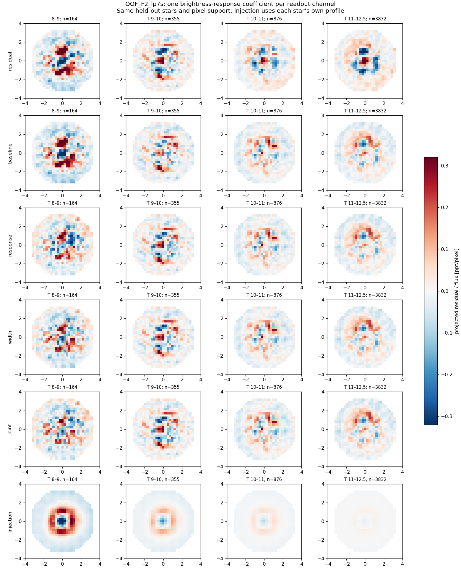
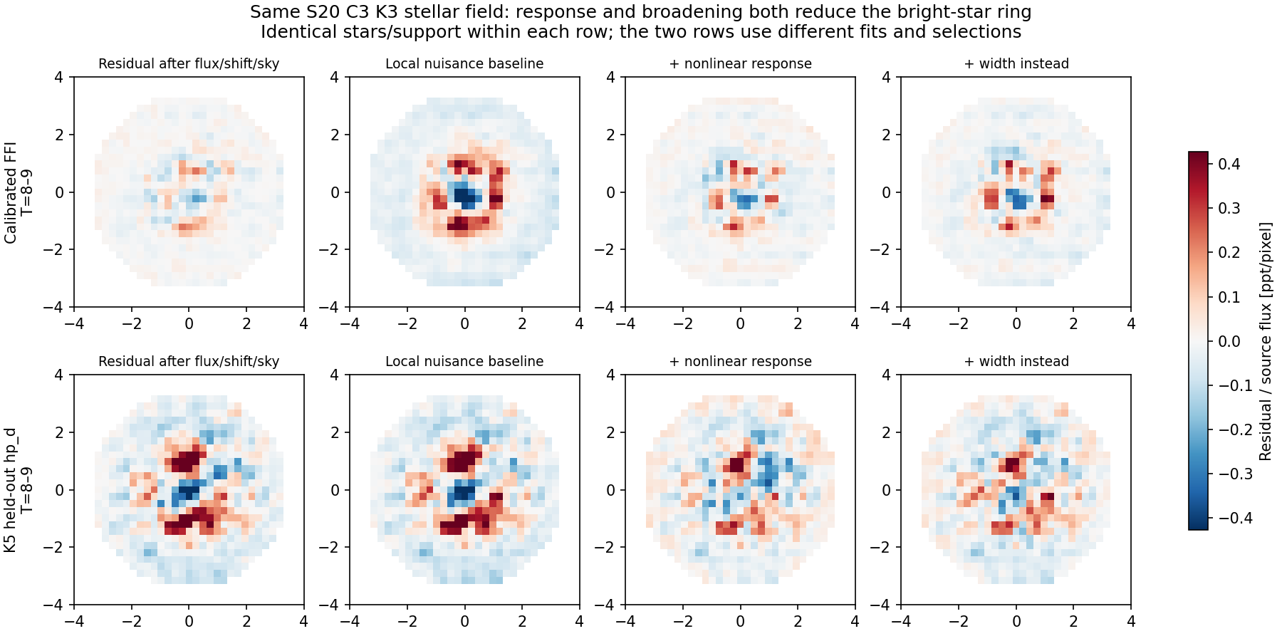 The proposed response correction changes the bright core/ring, but width changes have a similar effect. Remaining asymmetric structure is visible.
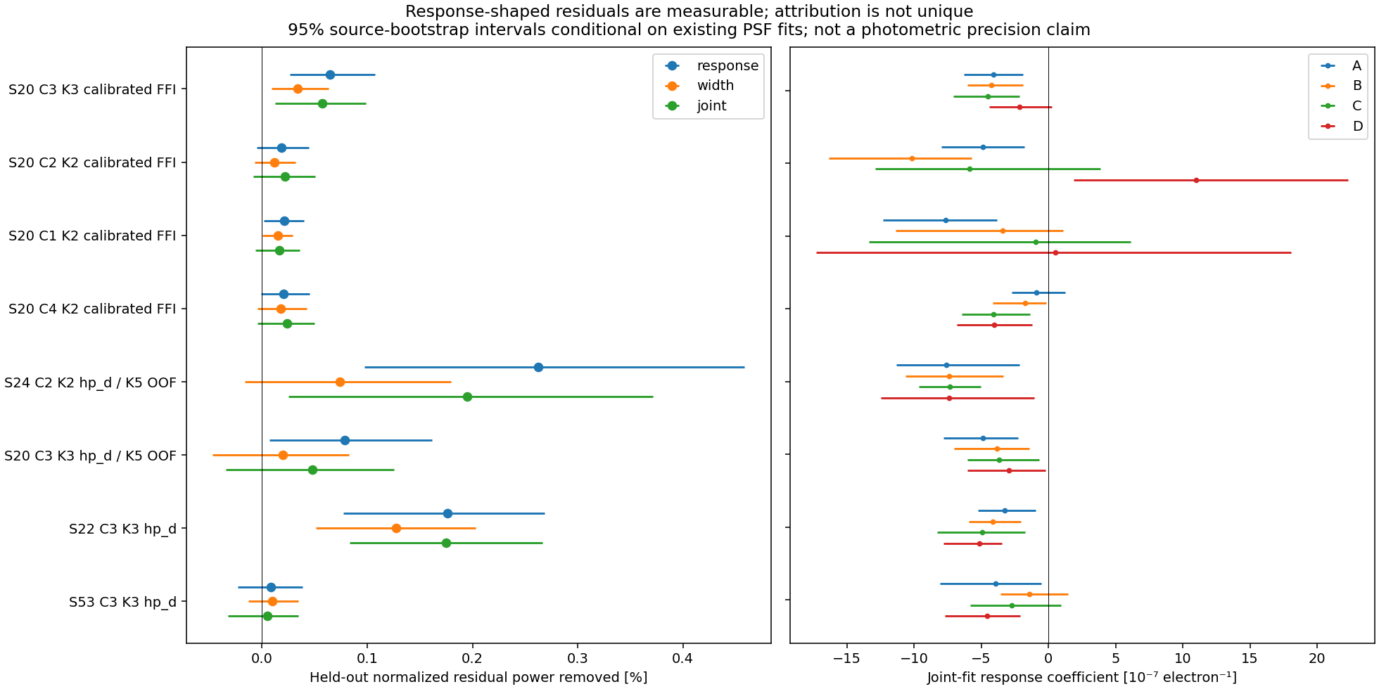 Percentages refer to held-out, normalized residual squared power after nuisance controls—not flux bias or photometric precision. 95% intervals are conditional source-bootstrap intervals.
| Dataset | Stars | Response gain | Width gain | Joint gain |
|---|
| S20 C3 K3 calibrated FFI | 5497 | 0.0649% | 0.0339% | 0.0572% |
| S20 C2 K2 calibrated FFI | 5524 | 0.0185% | 0.0117% | 0.0219% |
| S20 C1 K2 calibrated FFI | 5082 | 0.0212% | 0.0149% | 0.0164% |
| S20 C4 K2 calibrated FFI | 4962 | 0.0207% | 0.0179% | 0.0236% |
| S24 C2 K2 hp_d / K5 OOF | 5144 | 0.2627% | 0.0741% | 0.1952% |
| S20 C3 K3 hp_d / K5 OOF | 5227 | 0.0789% | 0.0197% | 0.0479% |
| S22 C3 K3 hp_d | 5331 | 0.1763% | 0.1276% | 0.1747% |
| S53 C3 K3 hp_d | 6315 | 0.0081% | 0.0097% | 0.0050% |
3. Validation, sector transfer and limitations
The first diagnostic used a patch-averaged profile for the response template. Injection into each star's own model exposed leakage into width; those exploratory results are superseded. Version 2 uses the star's own pixel model for the quadratic-response and flux terms. Exact response, width, joint and zero injections recover the supplied coefficients. Own-profile response injection also recovers the injected coefficient to numerical precision. These are conditional template/estimator tests, not proof of an independently known PSF or real detector response.
Additional controls add the known quarter-pixel interpolation-phase covariates. A response learned from S20 C3 K3 is then held fixed when testing S22 and S53 C3 K3, while only local nuisance shapes are fitted in the target. The same-epoch hp_d comparison is a processing comparison, not independent replication. Later-sector hp_d tests retain template and PSF-model confounds.
| Fixed S20 response applied to | Residual-power gain | Conditional 95% interval |
|---|
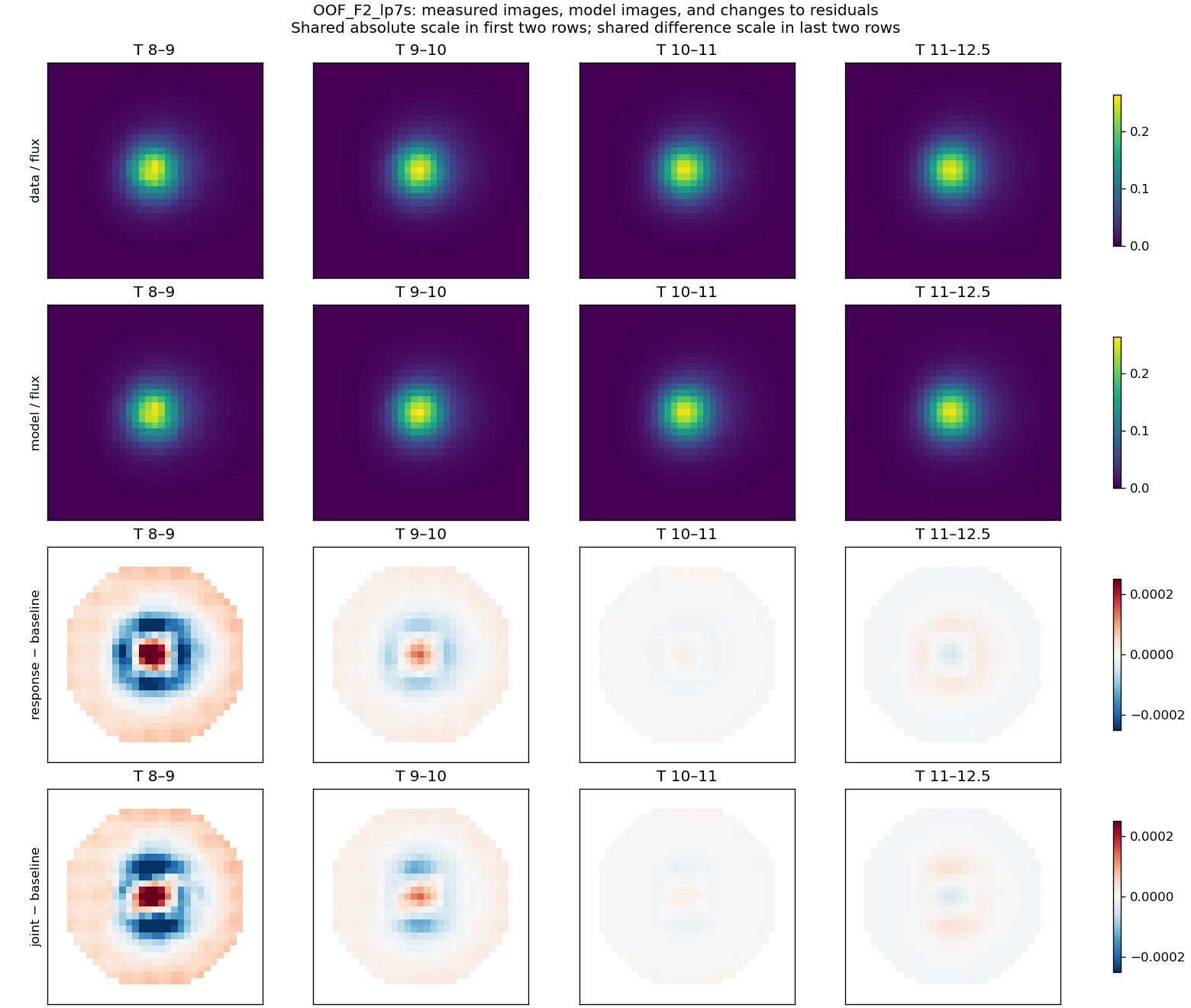
| OOF_F2_lp7s | 0.1547% | 0.0570 to 0.2449% |
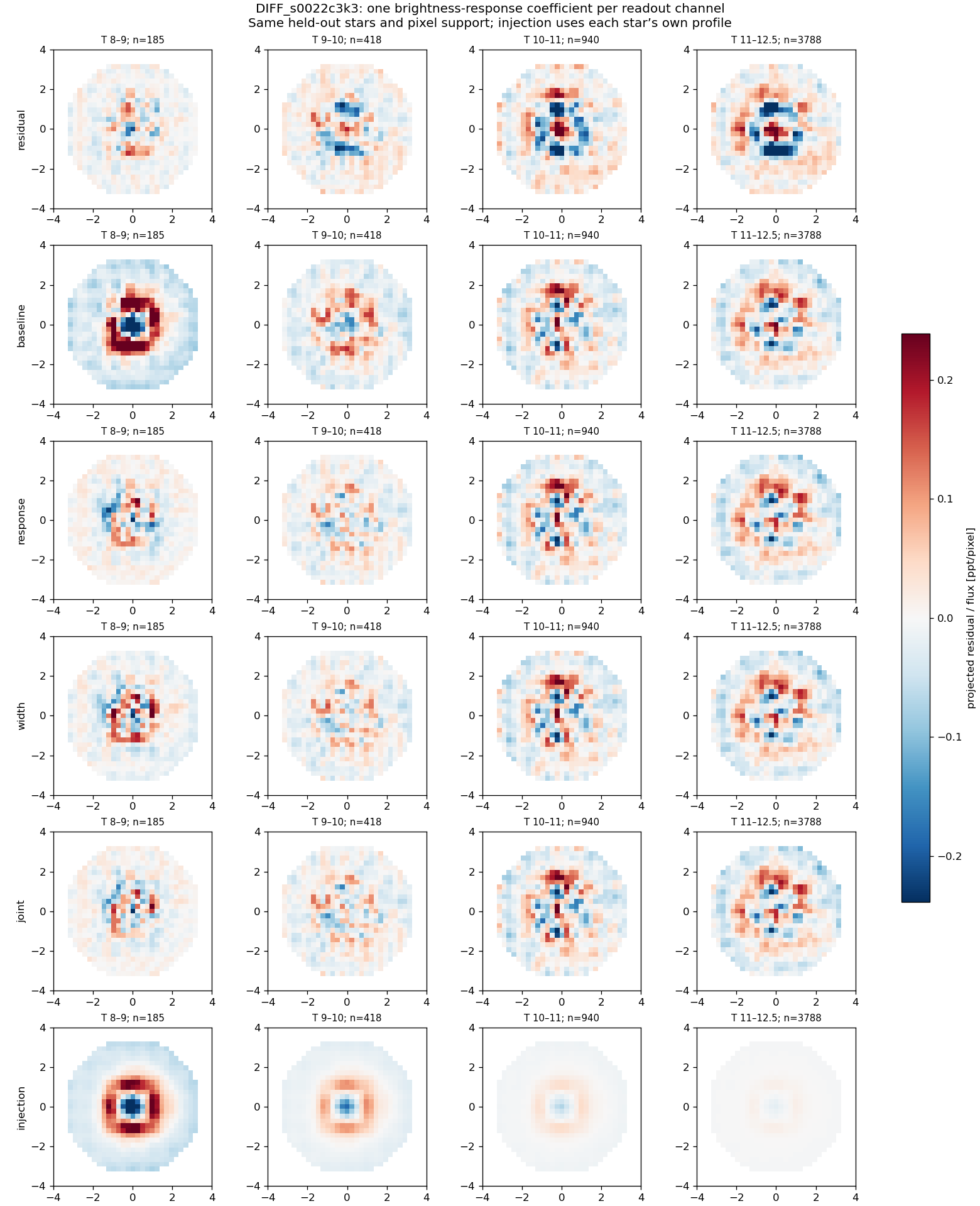
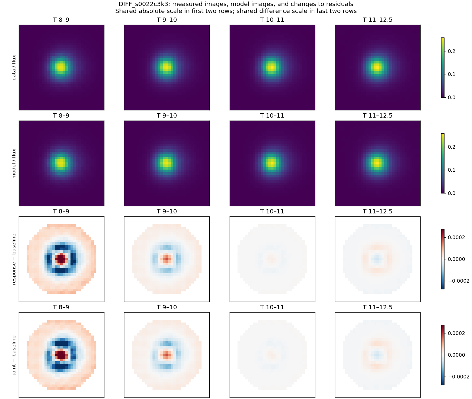
| DIFF_s0022c3k3 | 0.0907% | -0.0133 to 0.1670% |
| DIFF_s0053c3k3 | 0.0297% | -0.0062 to 0.0645% |
The S22 and S53 transfer intervals include zero: an independent-sector improvement is not established at this conditional 95% level. This is an acceptance failure for a universal correction, not proof that nonlinearity is absent.
OOF_F2_lp7s: images behind the fixed-response transfer score
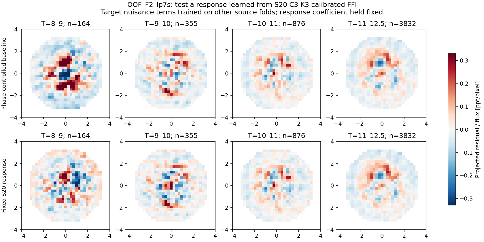 Phase-controlled target baseline and fixed S20 response on identical held-out stars/pixels. These images correspond to the transfer scores above, not the freely refitted response in the main gallery.
DIFF_s0022c3k3: images behind the fixed-response transfer score
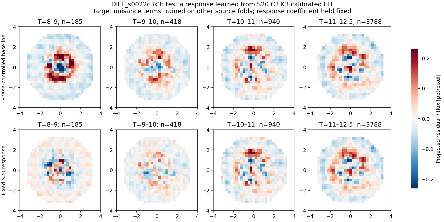 Phase-controlled target baseline and fixed S20 response on identical held-out stars/pixels. These images correspond to the transfer scores above, not the freely refitted response in the main gallery.
DIFF_s0053c3k3: images behind the fixed-response transfer score
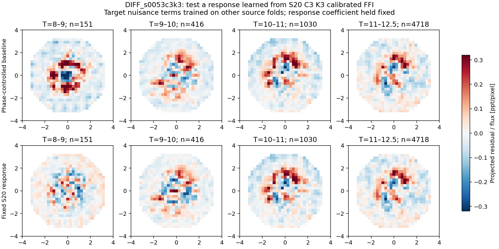 Phase-controlled target baseline and fixed S20 response on identical held-out stars/pixels. These images correspond to the transfer scores above, not the freely refitted response in the main gallery.
See full phase and transfer results. No transit/variability injection, temporal photometric preservation test, new nonlinear joint scene fit, or independent on-orbit response reference was completed. Accordingly, no pixel correction is approved by this investigation.
4. Complete image evidence
S20 C3 K3 calibrated FFI: complete residual and measured-image gallery
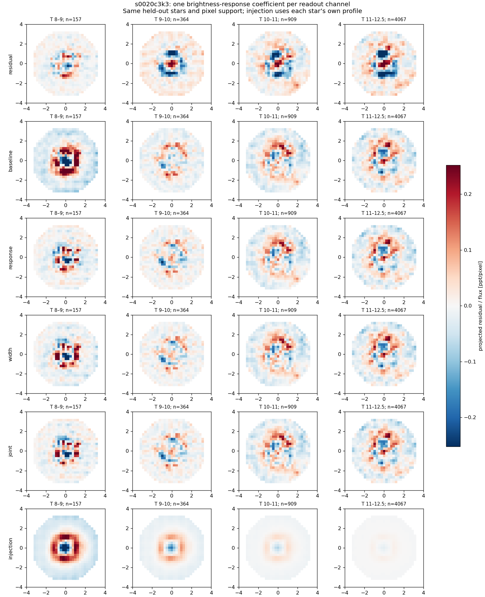 Six rows: original projected residual; nuisance baseline; added response; added width; joint; injected response. All panels use one residual scale. Equal-star means; each magnitude bin lists its count.
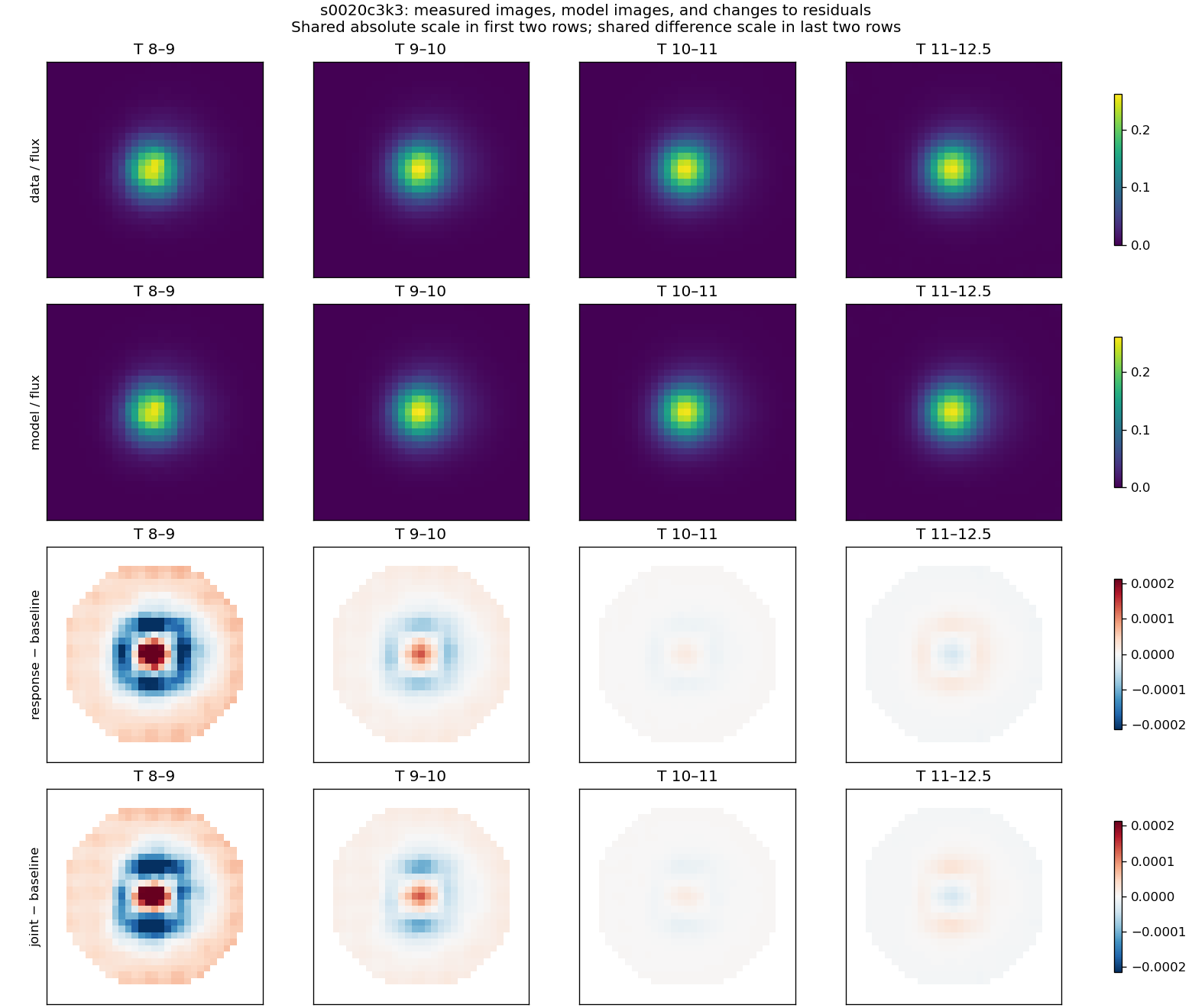 Actual data and model stacks above; response-minus-baseline and joint-minus-baseline residual differences below. Shared scales within each pair of rows.
S20 C2 K2 calibrated FFI: complete residual and measured-image gallery
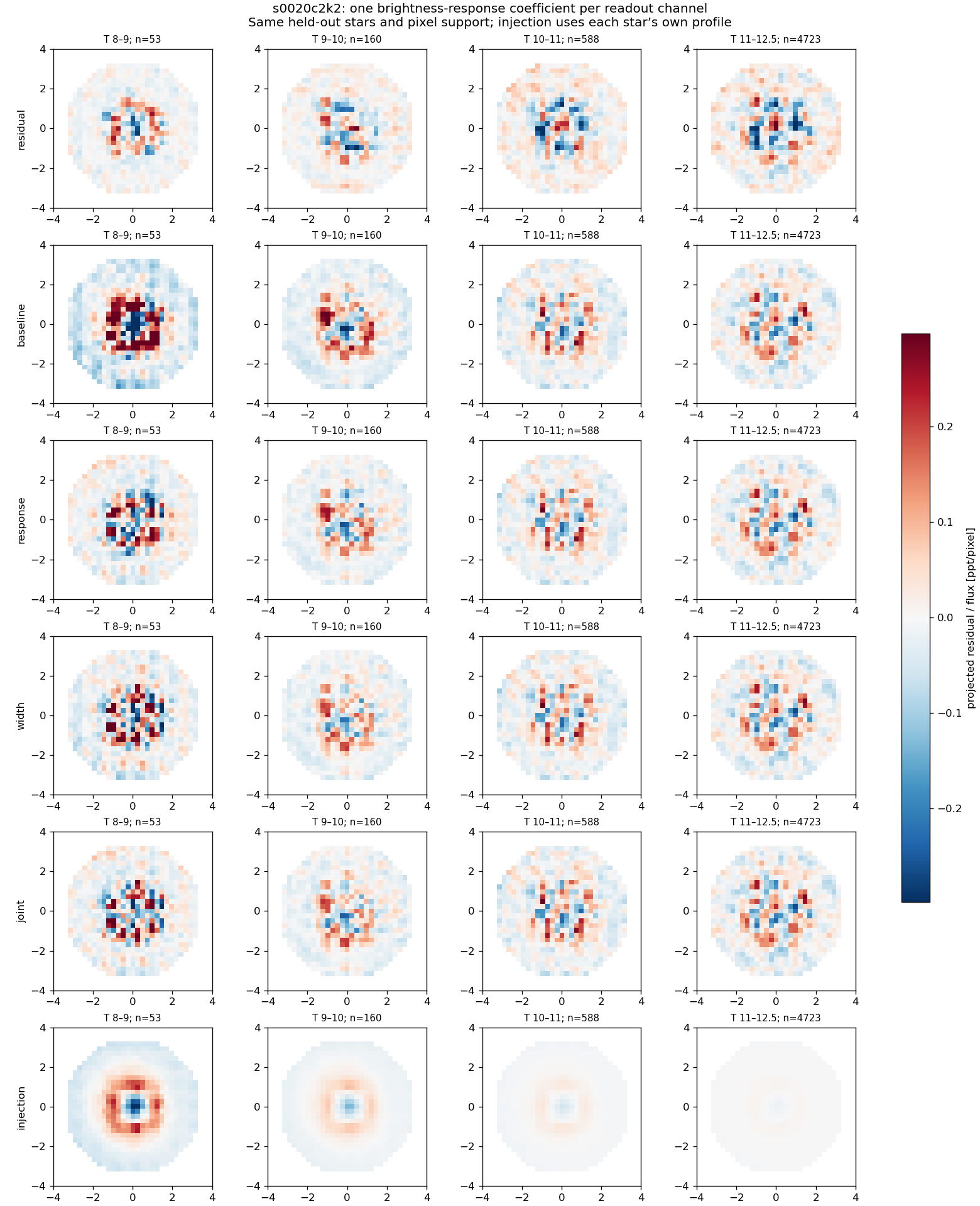 Six rows: original projected residual; nuisance baseline; added response; added width; joint; injected response. All panels use one residual scale. Equal-star means; each magnitude bin lists its count.
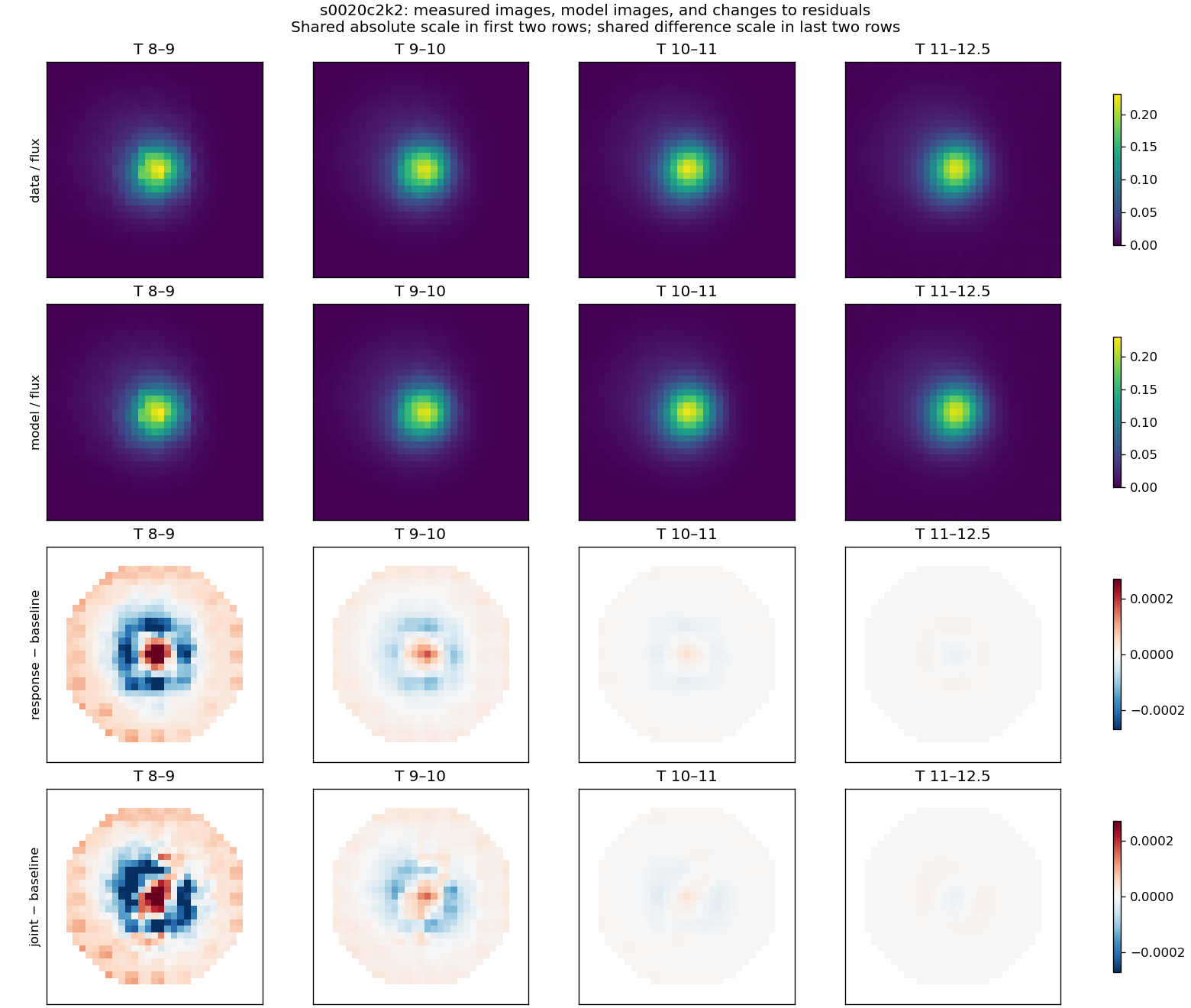 Actual data and model stacks above; response-minus-baseline and joint-minus-baseline residual differences below. Shared scales within each pair of rows.
S20 C1 K2 calibrated FFI: complete residual and measured-image gallery
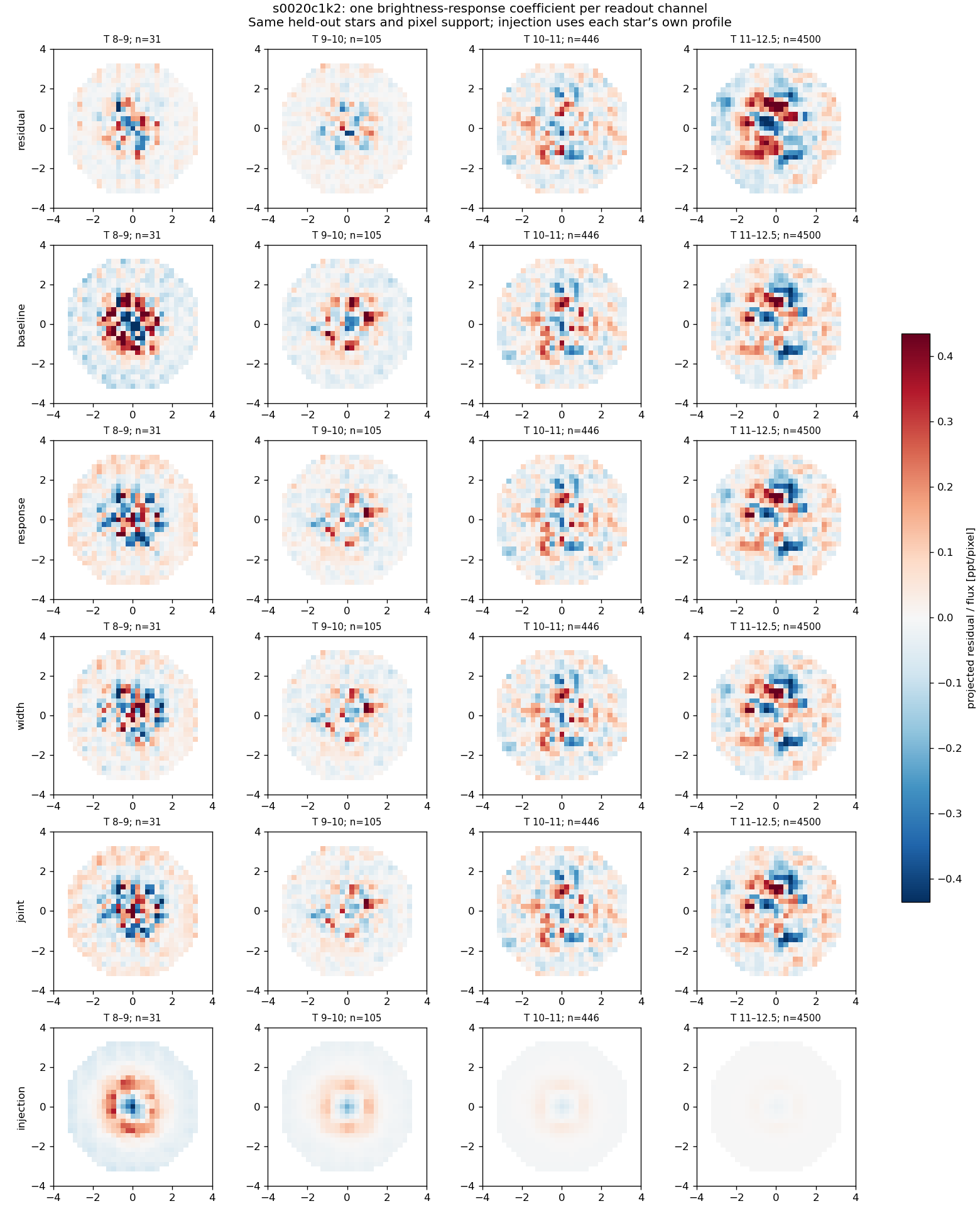 Six rows: original projected residual; nuisance baseline; added response; added width; joint; injected response. All panels use one residual scale. Equal-star means; each magnitude bin lists its count.
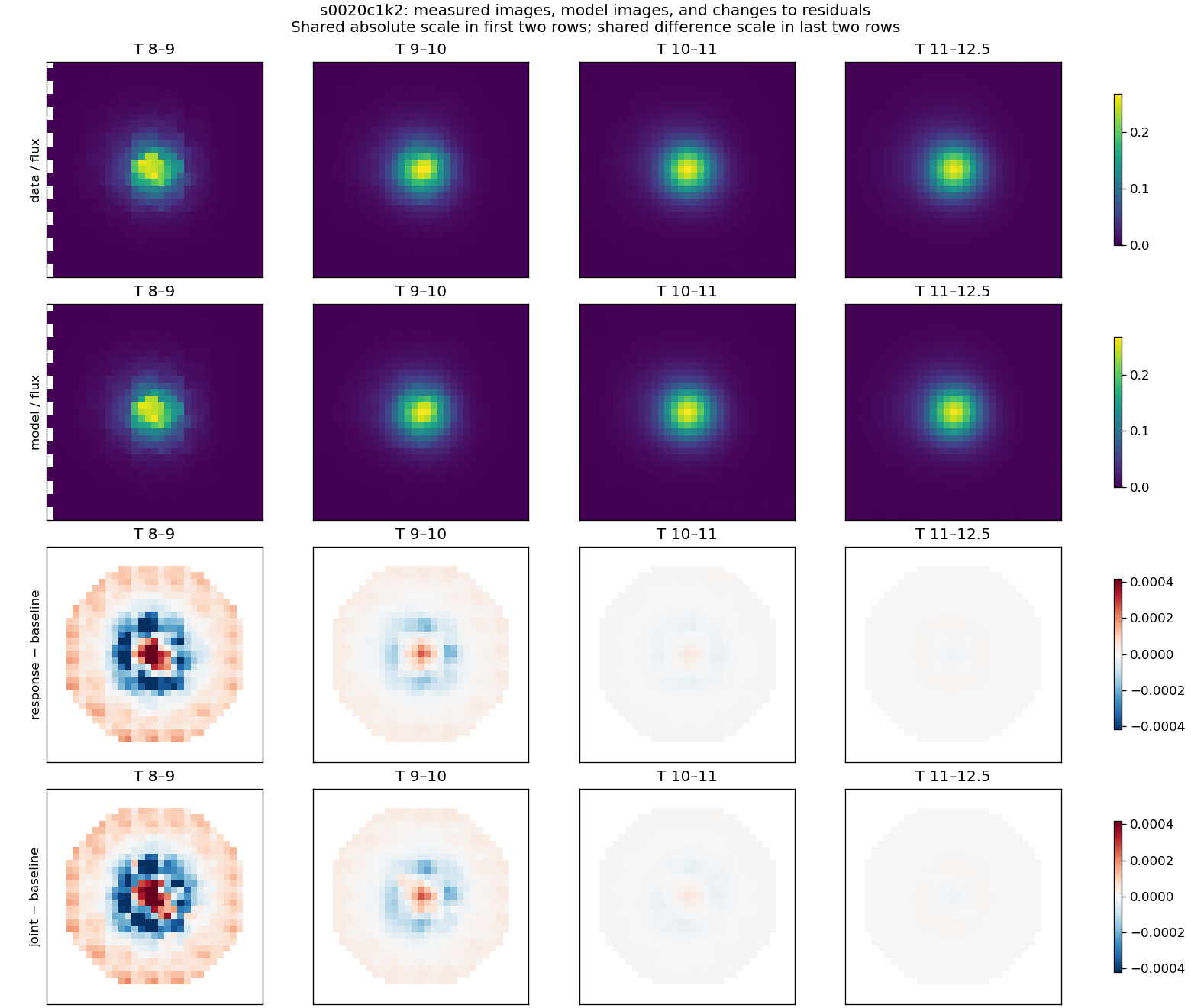 Actual data and model stacks above; response-minus-baseline and joint-minus-baseline residual differences below. Shared scales within each pair of rows.
S20 C4 K2 calibrated FFI: complete residual and measured-image gallery
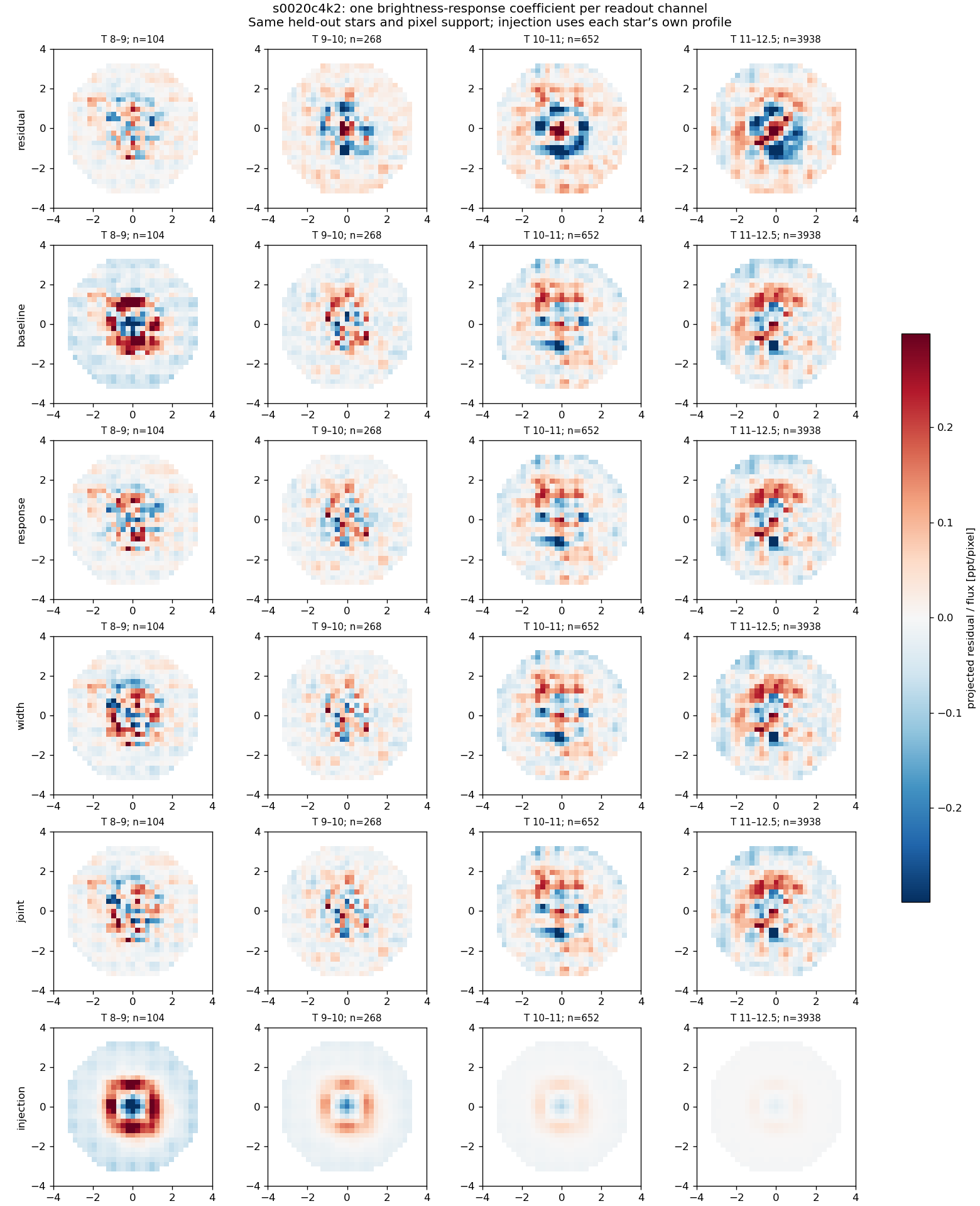 Six rows: original projected residual; nuisance baseline; added response; added width; joint; injected response. All panels use one residual scale. Equal-star means; each magnitude bin lists its count.
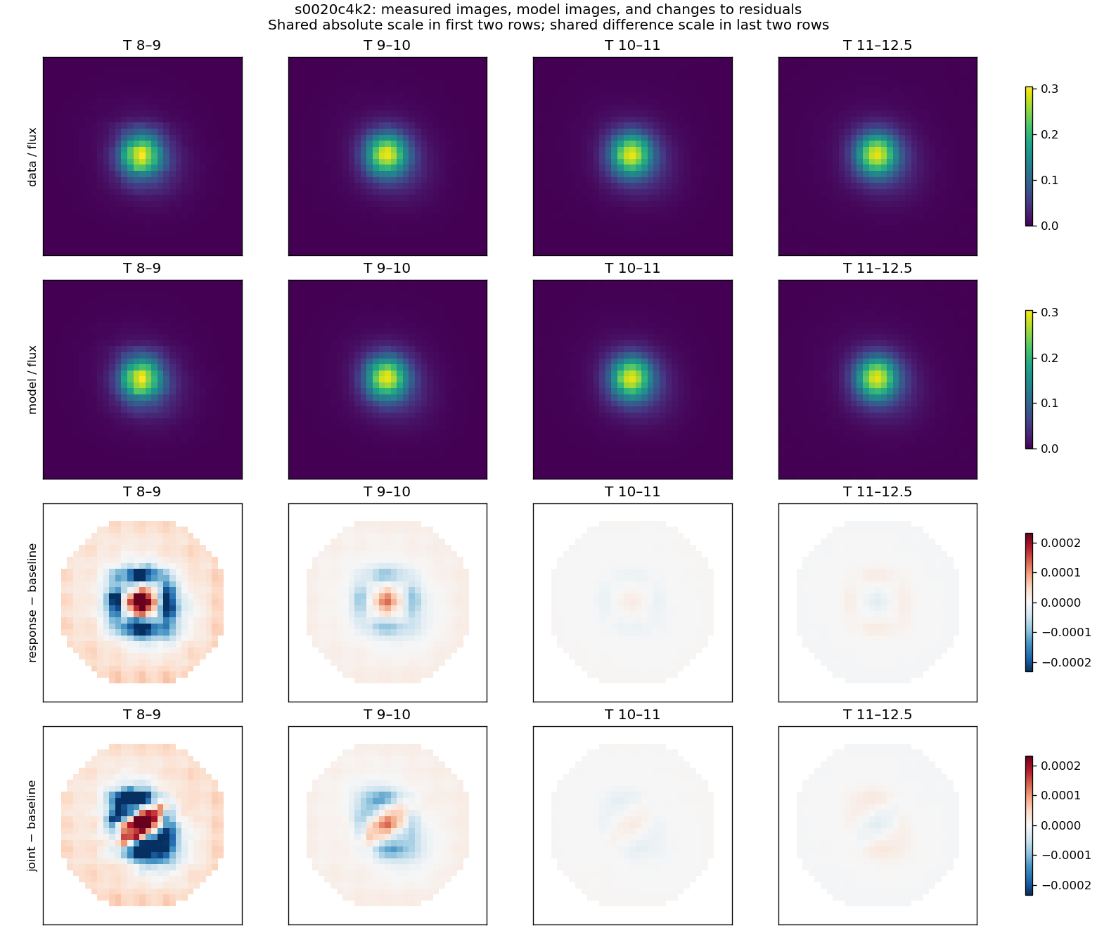 Actual data and model stacks above; response-minus-baseline and joint-minus-baseline residual differences below. Shared scales within each pair of rows.
S24 C2 K2 hp_d / K5 OOF: complete residual and measured-image gallery
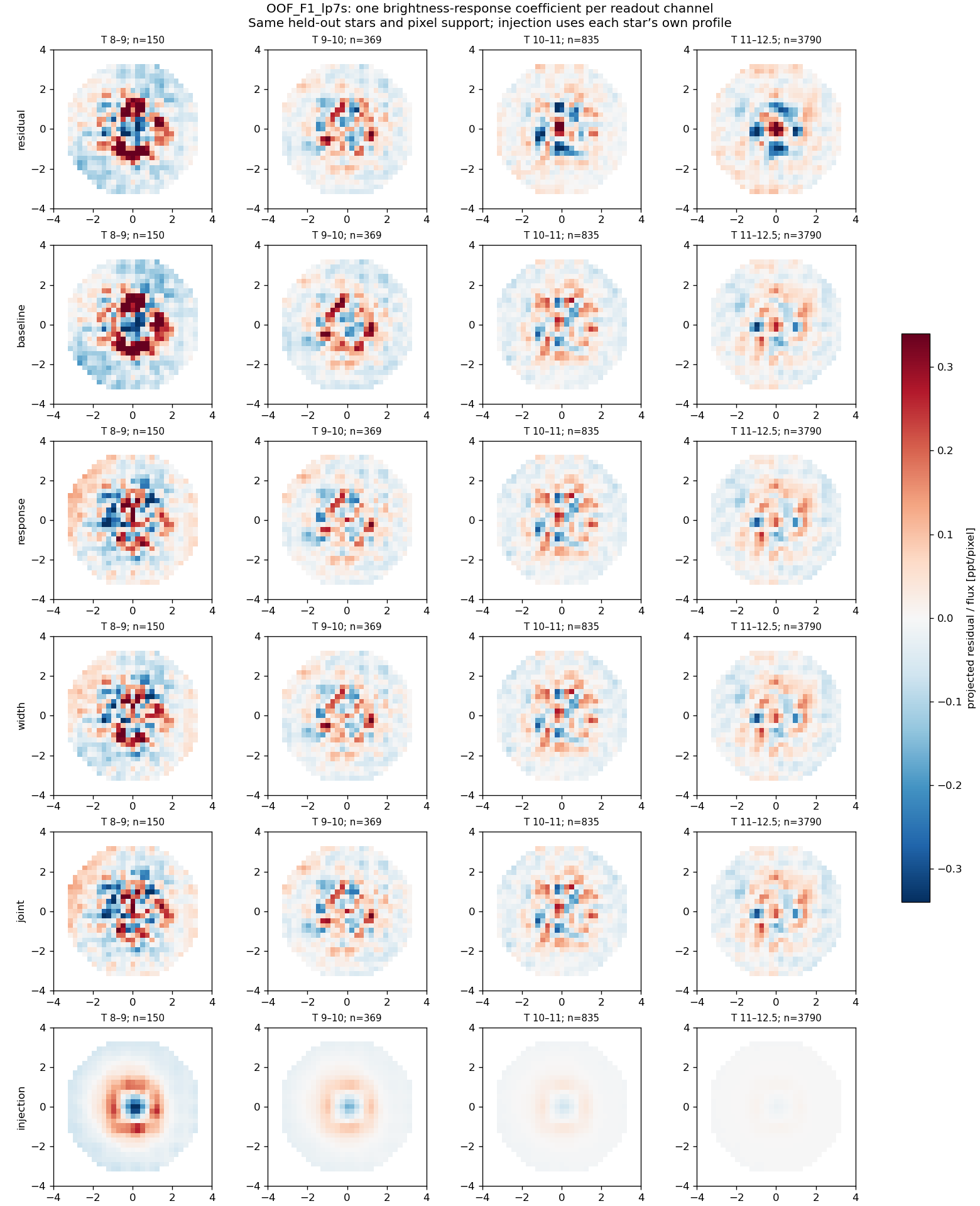 Six rows: original projected residual; nuisance baseline; added response; added width; joint; injected response. All panels use one residual scale. Equal-star means; each magnitude bin lists its count.
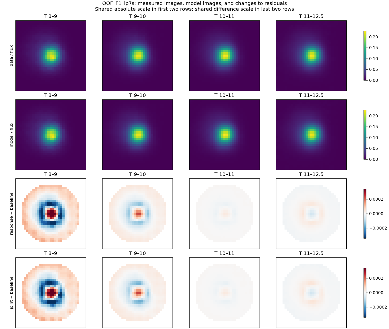 Actual data and model stacks above; response-minus-baseline and joint-minus-baseline residual differences below. Shared scales within each pair of rows.
S20 C3 K3 hp_d / K5 OOF: complete residual and measured-image gallery
 Six rows: original projected residual; nuisance baseline; added response; added width; joint; injected response. All panels use one residual scale. Equal-star means; each magnitude bin lists its count.
 Actual data and model stacks above; response-minus-baseline and joint-minus-baseline residual differences below. Shared scales within each pair of rows.
S22 C3 K3 hp_d: complete residual and measured-image gallery
 Six rows: original projected residual; nuisance baseline; added response; added width; joint; injected response. All panels use one residual scale. Equal-star means; each magnitude bin lists its count.
 Actual data and model stacks above; response-minus-baseline and joint-minus-baseline residual differences below. Shared scales within each pair of rows.
S53 C3 K3 hp_d: complete residual and measured-image gallery
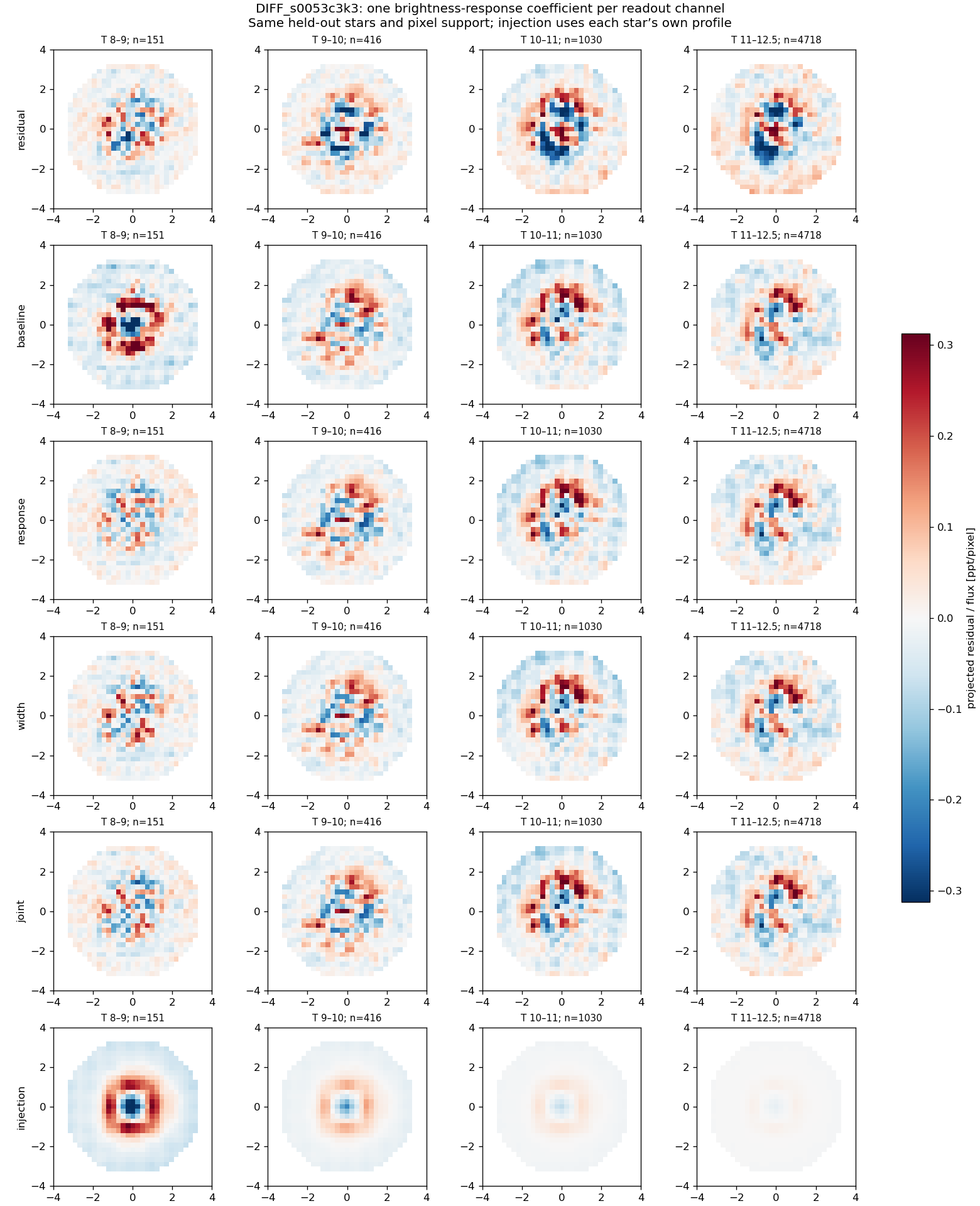 Six rows: original projected residual; nuisance baseline; added response; added width; joint; injected response. All panels use one residual scale. Equal-star means; each magnitude bin lists its count.
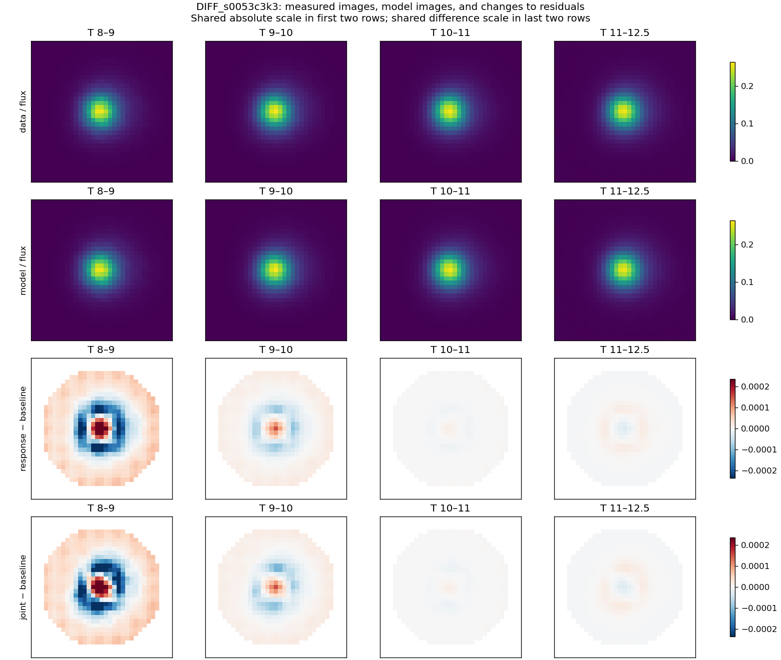 Actual data and model stacks above; response-minus-baseline and joint-minus-baseline residual differences below. Shared scales within each pair of rows.
s0020c3k3: colour × magnitude × 3×3 CCD controls
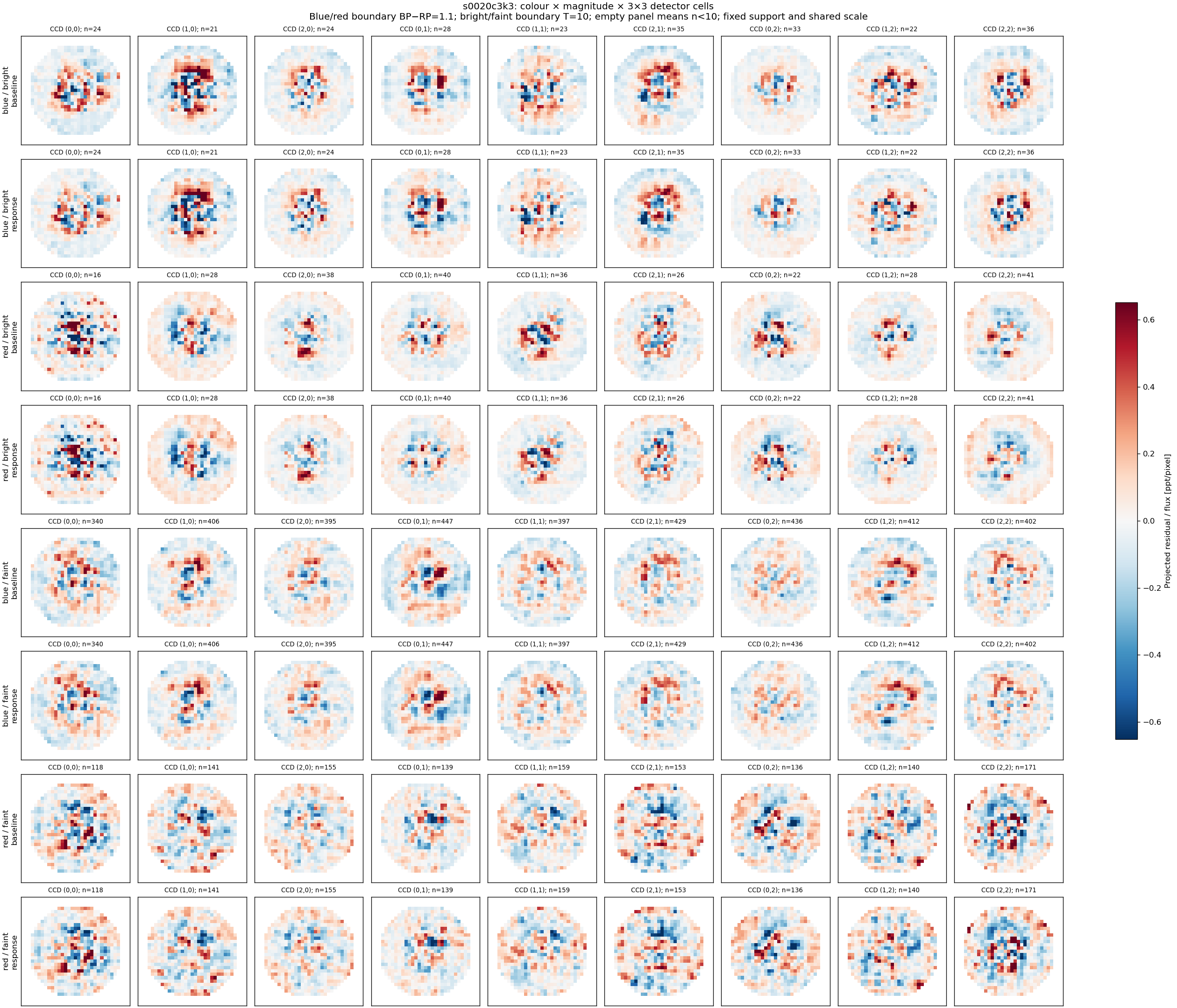 Identical before/after support, fixed colour/magnitude thresholds, shared scale and explicit bin counts. Small bins are blank, not evidence of closure.
OOF_F1_lp7s: colour × magnitude × 3×3 CCD controls
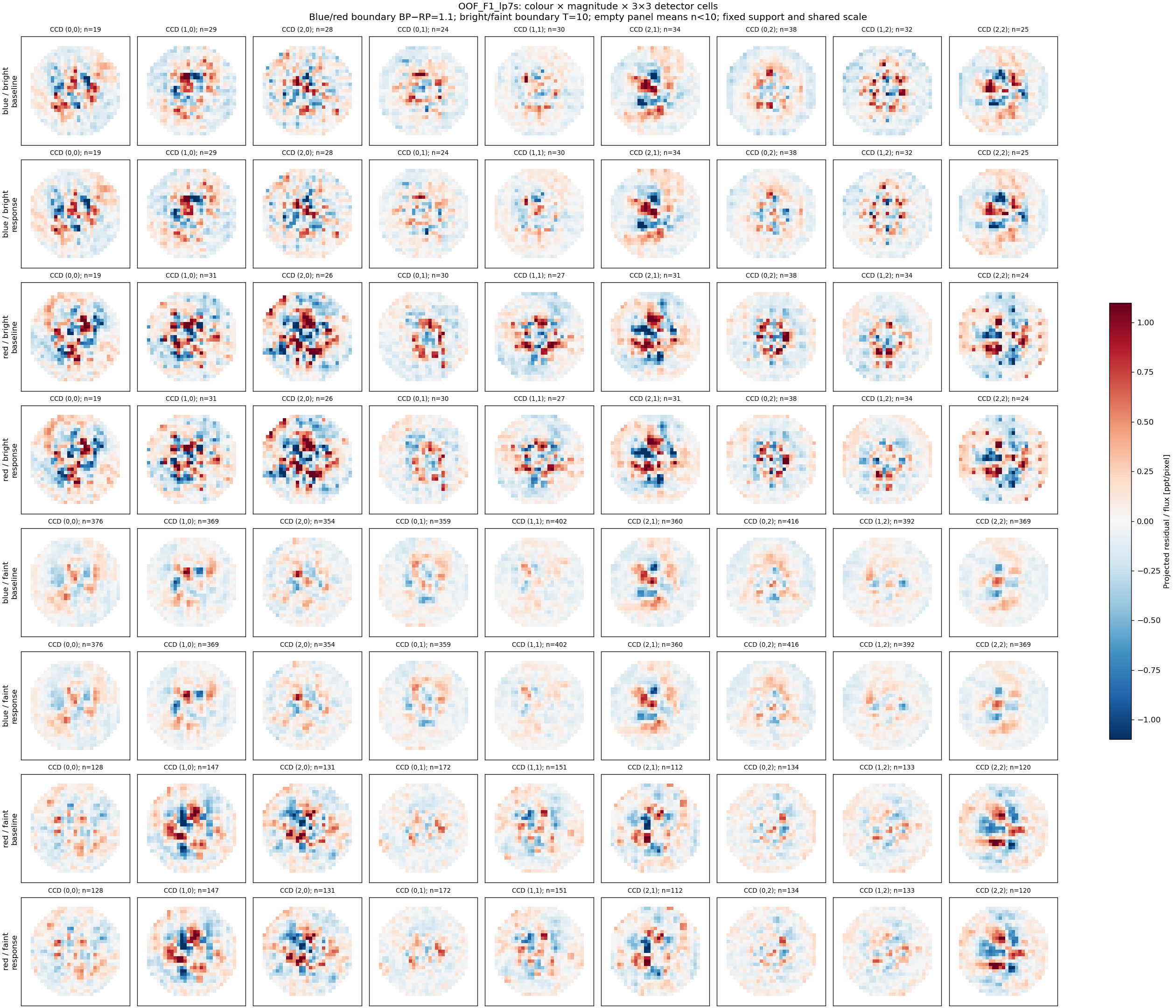 Identical before/after support, fixed colour/magnitude thresholds, shared scale and explicit bin counts. Small bins are blank, not evidence of closure.
OOF_F2_lp7s: colour × magnitude × 3×3 CCD controls
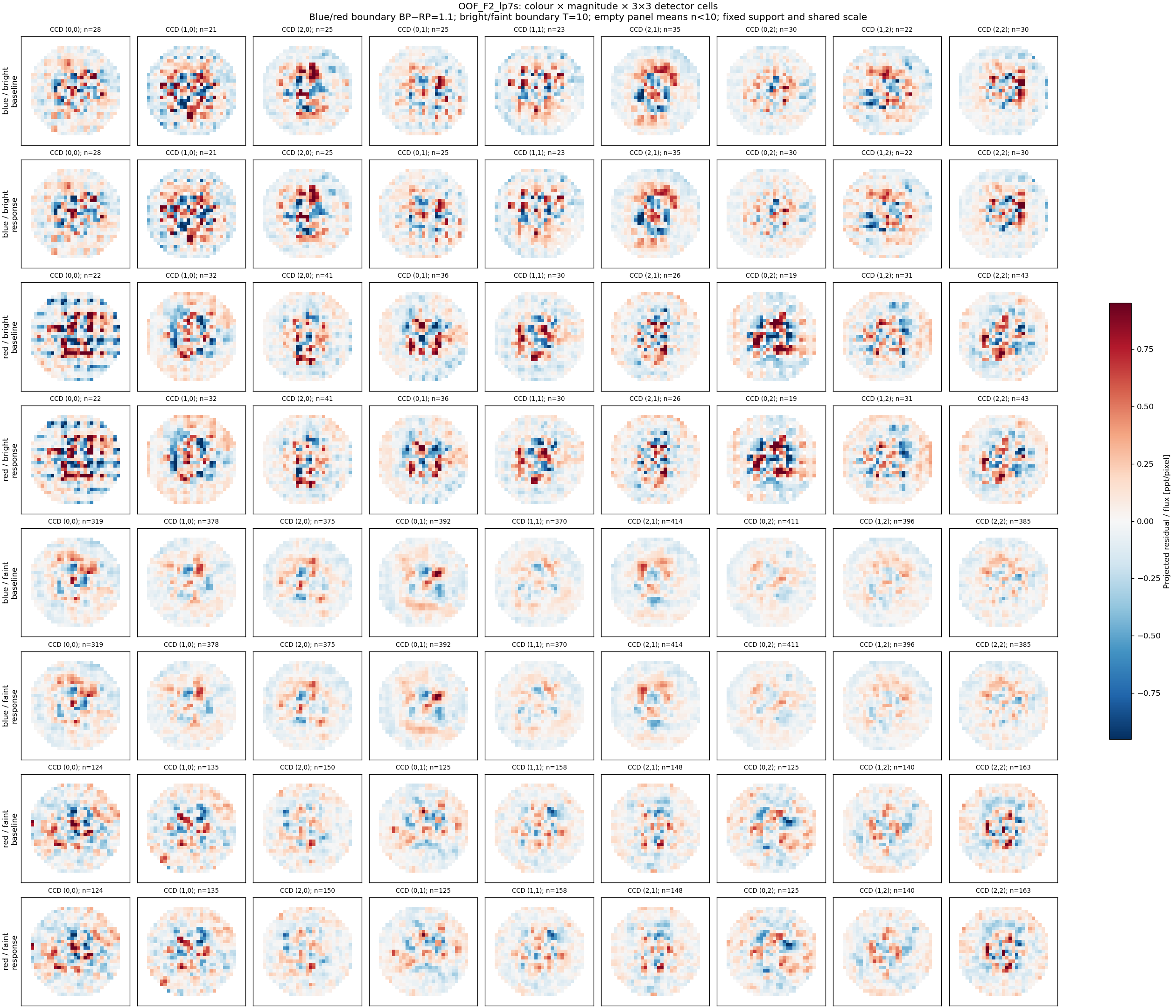 Identical before/after support, fixed colour/magnitude thresholds, shared scale and explicit bin counts. Small bins are blank, not evidence of closure.
Conclusion
Nonlinearity remains a plausible contributor to peak flattening, but is not established as the cause of all the observed effects. Correct application of a reference curve and physical correctness of that curve are different questions. The tested application is accurate; the stellar residuals support a small response-shaped component whose attribution remains mixed with PSF shape and processing errors. A wholesale inverse correction is not justified. The next decisive step is a joint response-plus-PSF fit on calibrated, unsubtracted images across multiple epochs, with independent source/epoch holdouts and photometric signal-preservation tests—or an independent detector response reference. The diagnostic implementation is repaired and archived; production science pixels are unchanged.
Reproducibility and sources
Run record and exact commands · Input/code manifest. All output is under /astro/armin/koji/syndiff/dev_runs/nonlinearity_peak_20261002/. Code backup branch: codex/nonlinearity-peak-20261002. Final shape evidence is in v2/; root-level exploratory shape results are superseded.
TESS Instrument Handbook, §§6.4.2 and 9.5.1 · Pinned independent TICA response implementation · MAST reference models.