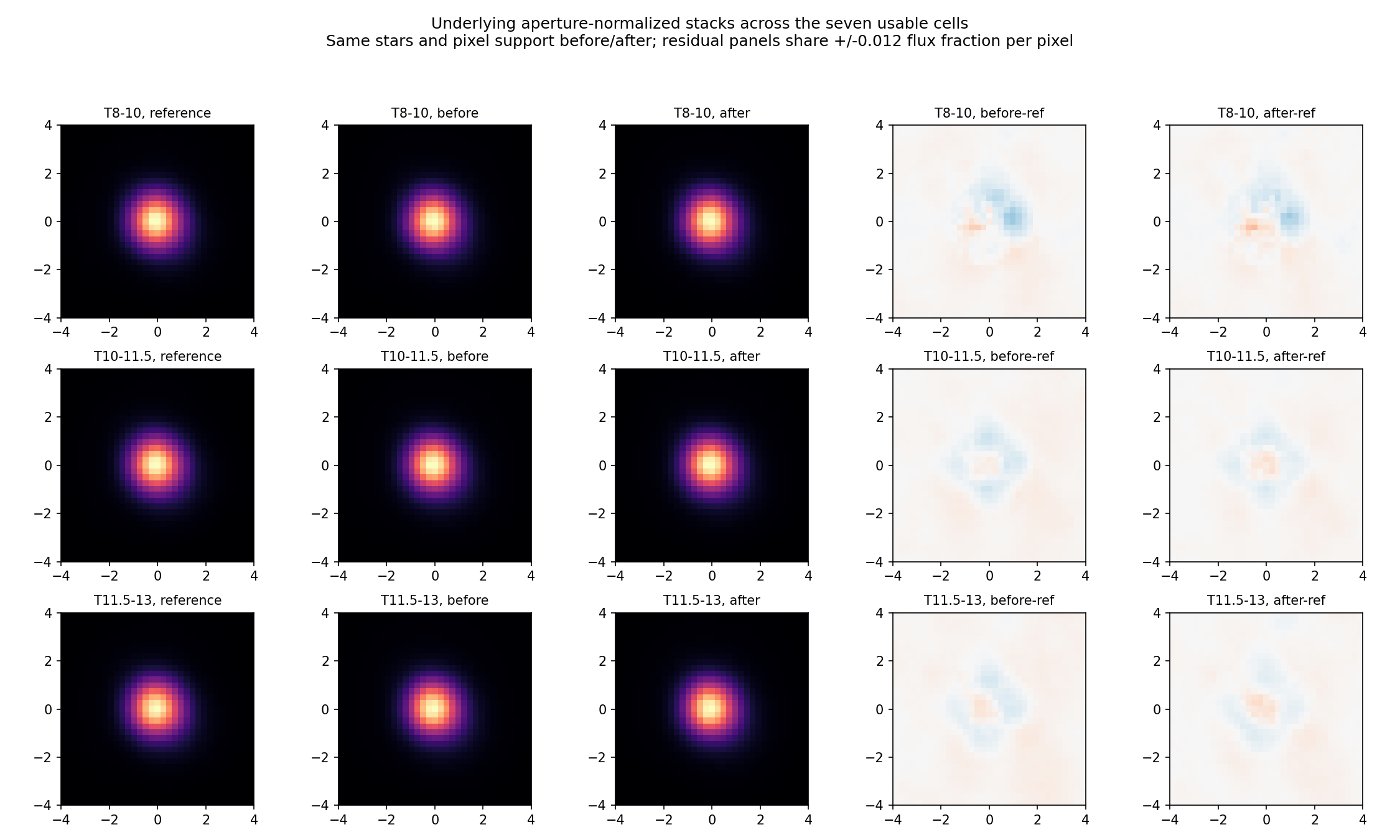
2026-10-02. Completed bounded real-image experiment. Question: after subtracting faint neighbours using a faint-star ePSF, do bright-star profiles become the same as the faint reference, across magnitude and detector position?
No general improvement is established in this pilot. The median paired native-pixel shape-error ratio is consistent with one in all three magnitude bins for the moderate and tighter amplitude settings. The spatial/magnitude images retain asymmetric differences from the faint reference after subtraction. Weak amplitude regularization worsens the typical error in the two fainter bins. Some individual stamps improve, but that is not a population-wide removal of magnitude dependence.
This is actual RAW-TESS-trained ePSF creation and subtraction on actual hp_d images, followed by empirical phase-aligned PSF stacks. It is not the earlier shared-PS1-profile injection test. It is also not a full production joint ePSF/WCS retrain, a complete PS1-derived source inventory, or proof that the remaining structure is a physical brighter-fatter effect.
C4 is sector 23, camera 4, CCD 2, FFI `tess2020087042920`. Seven detector cells have usable independently trained faint references, using 108 calibration stars in total. Cell 7 had only five usable stars and was not scored; cell 8 met a centring stop criterion but its last profile update was still 8.6% of peak, so it was excluded. The retained cells' last profile changes were below 1% of peak. This is a stability check, not a complete calibration uncertainty estimate.
The common science population is 506 stars present with valid positive aperture normalization in all amplitude variants. The table uses median per-star after/before native-pixel shape RMS, on exactly the same valid pixels inside a three-pixel radius. A ratio below one means closer to the faint reference. The intervals are 95% spatial-block bootstrap intervals, conditional on these fitted references; they do not propagate reference-training uncertainty or turn one FFI into independent fields.
| Catalogue T magnitude | Common stars | Moderate-amplitude after/before ratio | 95% block interval |
| 8–10 | 68 | 1.0001 | 0.9983–1.0016 |
| 10–11.5 | 204 | 1.0003 | 0.9932–1.0124 |
| 11.5–13 | 234 | 1.0072 | 0.9970–1.0290 |

Each detector cell has three magnitude rows. Columns show the faint reference, bright-star profile before subtraction, after subtraction, after minus reference, and after minus before. Absolute and difference panels each use shared scales. Both unsupported detector cells are explicitly marked. The figure and table use the common population across all amplitude settings. These are median empirical ePSF stacks on a common quarter-pixel display grid, not separately trained high-dimensional PSFs in sparse bright bins.
The remaining differences are visibly asymmetric/dipolar in several bins. A scalar width alone would conceal that morphology. Bright and faint targets also sample colour and sub-cell position differently; this experiment does not uniquely isolate an intrinsic magnitude law.
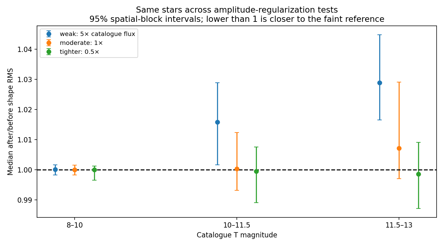
The amplitude factors above are widths of a zero-centred residual-flux regularizer, not a measured catalogue-flux uncertainty or a positive full-source prior. The moderate setting uses one nominal catalogue flux as its width; tighter uses half, weak uses five times. The ordinary zero of the ratio axis is not meaningful here: the relevant null is one. All intervals for moderate/tighter settings include one. Weak regularization produces increased median shape error for the two fainter bins. Shifting faint-source positions by 90 degrees around the target gives worse common-support median ratios than the corresponding real-position arm, but the real-position arm still does not generally improve the shape.
A separate local Photutils EPSFBuilder fit was made in each populated 3x3 CCD cell from RAW TESS stamps of stars with catalogue T11.5–13 and cont4<0.03. cont4 is the available catalogue neighbour/target flux ratio within four pixels, not a purity guarantee. Saturation, bleed, inherited exclusion, core finite-pixel and strap cuts were applied. Pixels within 2.5 native pixels of neighbours brighter than 0.005 of the target were masked; an outer clean ring supplied the initial background. Cells needed at least six usable calibration stars.
The builder used 4x sampling, a 65x65 grid, quadratic smoothing, a five-pixel centroid-fitting box, centre tolerance 0.003 native pixel and a cap of 15 iterations. Retained references stopped in four to eight iterations, with the shape-stability qualification above. Calibration and evaluation lie on disjoint guarded 128-pixel tiles; source IDs and stamp origins were checked. The calibrated profile is a local cell average, not a continuously spatial/colour-dependent truth PSF. Core isolation does not eliminate unresolved background or all outer-wing contamination.
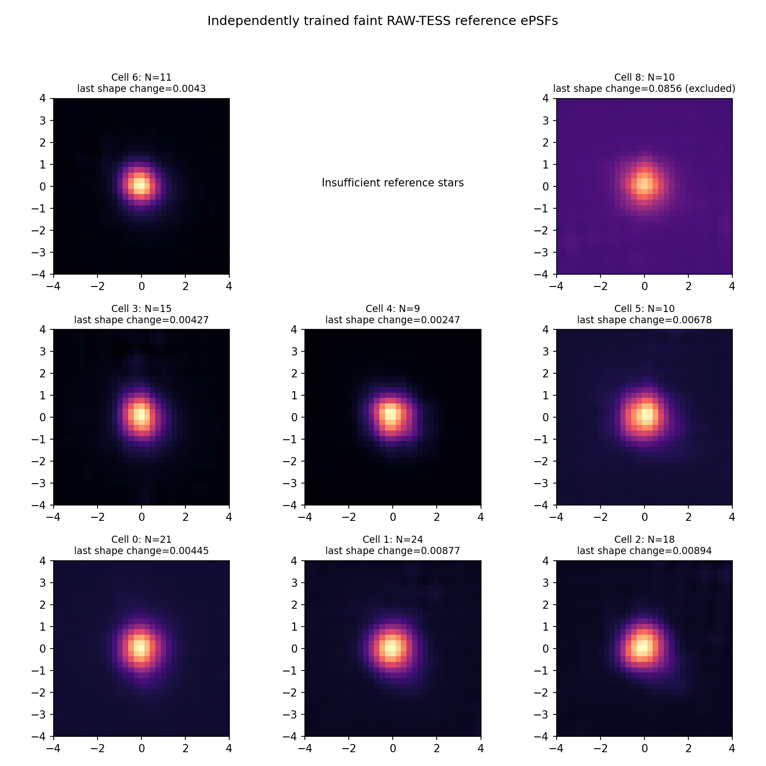
The first attempted local B-spline reference fit was unstable. It was stopped and its checkpoints/log preserved in `failed_bfw_reference/`; no final science result uses it. Photutils empirical references replaced that estimator. The initial science trial also capped neighbour lists; it is archived at the run root and is superseded by the uncapped `full_catalogue*` comparisons. Reference cell 8 is excluded in the latter comparisons. These corrections are part of the record rather than hidden failures.
Positions and nominal brightnesses come from the existing Gaia neighbour arrays attached to the atlas stamps. All available finite-brightness catalogue entries within nine pixels in each coordinate enter the final local model; there is no final top-N cap or relative-flux cutoff. The separately retrieved PS1 pilot catalogues are not used as calibrated flux truth here. Catalogue incompleteness remains a limitation.
The target has flux, first- and second-derivative shape terms, and a local plane in the linear fit, so the nuisance amplitudes are not forced to explain every target-width difference. Both bright and faint neighbours are fitted simultaneously. Neighbour amplitudes are signed residual fluxes in hp_d: a partially retained template can leave signed residual light. This approximates a residual source by a scaled faint TESS PSF; it is not the exact full-TESS-minus-retained-PS1 response and cannot represent every partial-removal shape.
Here $Q$ is the dimensionless fitted objective; $H$ is the active checkerboard training half of a stamp; $D_p$ is hp_d in e/s per native pixel; $m_p$ is its target, neighbour and plane model in the same units; $V_p$ is the unchanged saved pixel variance; $g_j$ is the fitted signed residual amplitude of neighbour $j$ in e/s; $F_j$ is its nominal Gaia-derived TESS flux in e/s; and $a$ is the chosen regularization factor (5, 1 or 0.5). The nominal conversion is the inherited 15000 e/s at T=10 convention, not a new calibration. A tiny numerical diagonal stabilization is also applied. The prior mean is zero and negative amplitudes are allowed.
Amplitudes fitted on one checkerboard half predict the other; the halves are swapped to assemble the output. The common target centroid was first estimated on the entire original stamp, so this is conditional cross-prediction, not completely blind pixel validation. The PSF reference itself uses disjoint stars/pixels. The original data/noise/masks are held fixed; subtraction does not remove photon noise. Existing historical selection masks are inherited in both arms.
For profile comparison, both images are normalized using the same aperture definition:
Here $s$ labels a target; $p,q$ label native pixels; $B_s$ is the fitted background plane; $L_s$ is the fitted bright-neighbour contribution; $N_s$ is the fitted contribution of neighbours with catalogue T>=13; all images have e/s per pixel units. The same $B_s,L_s$ are retained before and after. $A_s$ is the set of unchanged valid pixels within radius three of the common centre. $b=0$ denotes before and $b=1$ after; $I_s$ is the fraction of the aperture flux per native pixel. The faint reference is normalized on those exact pixels too. Nonpositive/nonfinite denominators are excluded consistently, and the main statistic intersects source IDs across all variants.
Native-pixel RMS against the reference is measured before interpolation. The display stacks interpolate all arms and reference identically to a quarter-pixel grid. Early plots divided by fitted target flux; their prominent central excess was substantially normalization-dependent. Aperture-normalized shape results above take precedence. Interpolated-RMS summaries and pooled quadratic errors are retained as diagnostics, but can give different impressions because smoothing and a few poorly deblended/low-denominator cases affect them. They are not substituted for the paired native-pixel statistic.
1. Faint-source positions rotated by 90 degrees provide a wrong-position control. Their amplitudes are refitted; the common bright-neighbour/background subtraction remains that of the real-position fit. This is a position sensitivity test, not an independent full null for every nuisance component.
2. A known width coefficient of 0.02 pixel² was added in the target Laplacian column while rendering catalogue neighbours. For moderate regularization, 129 cases had median recovered width 0.01999973 pixel²; the largest absolute error was 0.002522 pixel². Thus typical recovery is close, but some crowded cases transfer appreciable shape into nuisance amplitudes. This test uses the same linear template family for injection/recovery; it does not independently validate real PSF shape, noise, or arbitrary morphology.
3. All shape conclusions are restricted to this C4 FFI and the scored cells/population. No uncertainty interval here proves all real magnitude-dependent effects have been eliminated.
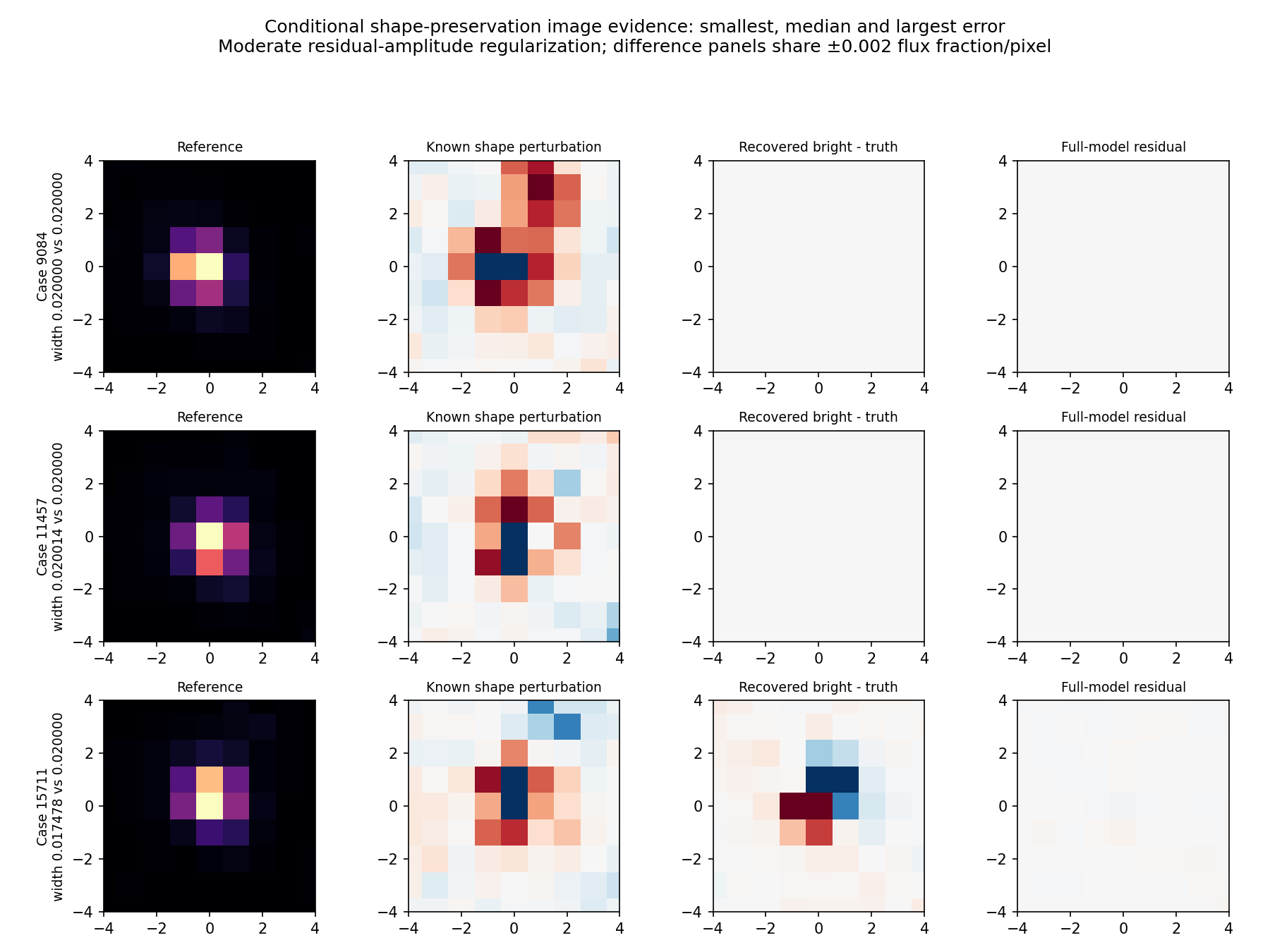
The three null examples are selected by smallest, median and largest width-recovery error. They show the reference, injected shape perturbation, recovered-primary-minus-truth image, and full-model residual on a shared difference scale. The worst case illustrates why a small overall residual does not guarantee correct allocation of source shape.
Absolute and cell-relative grids were generated and inspected for all subtraction variants and the faint RAW calibration set. They are added to the existing shared comparison page at http://localhost:18888/residual-grids/resgrid.html. The external Claude Artifact mirror could not be republished because no Artifact publishing tool is available.
The standard helper uses fitted-flux magnitude bins 8–10, 10–12, 12–13 and BP-RP colour bins. The main figures use fixed catalogue bins 8–10, 10–11.5, 11.5–13 and matched aperture normalization. These diagnostics therefore have different denominators and must not be read as interchangeable metrics. Empty colour/spatial bins mean insufficient data, not zero residual. Calibration-set grids are training checks, not held-out validation.
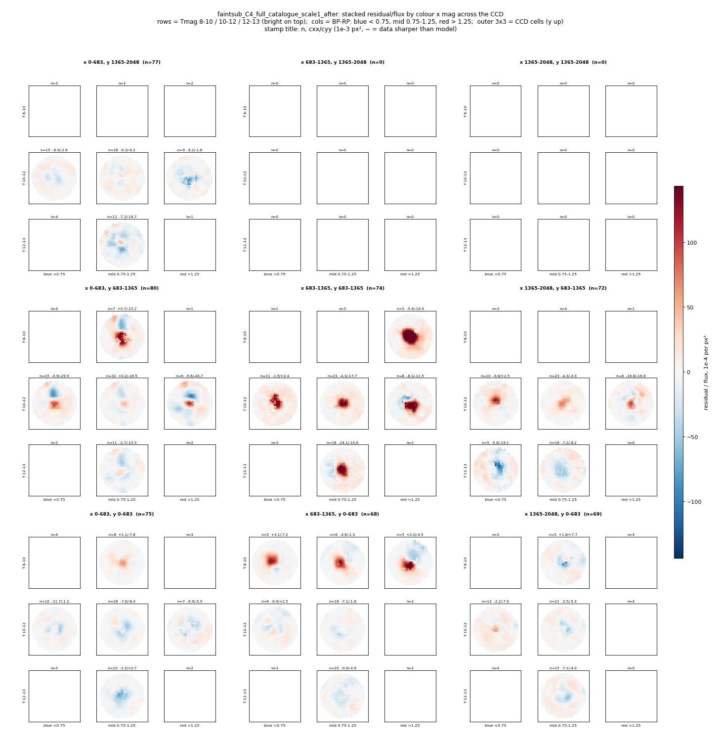
Run: `/astro/armin/koji/syndiff/dev_runs/neighbour_subtracted_epsf_20261002/`. Code is on `codex/ps1-stage-trace` in the nested dev worktree. Core inputs are `/astro/armin/koji/syndiff/dev_runs/epsf_atlas_20261001/stamps_v2/C4*` and `stamps_hpd/C4.npz`. `inputs.json`, per-variant input records, calibration checkpoints, native/raster stamps and per-star tables retain the exact samples and code hashes. `tables/common_support_summary.json` and `tables/common_ids.json` are the primary summary and common population.
After activating syndiff, with OPENBLAS_NUM_THREADS=1 and OMP_NUM_THREADS=1:
NEIGHBOUR_FULL=1 NEIGHBOUR_SCALE=1 python code/faint_subtracted_epsf.py
# Repeat with scales 5 and 0.5 for sensitivity.
SHAPE_VARIANT=full_catalogue_scale1 python code/faintsub_shape_checks.py
python code/faintsub_finalize.py
COMMON_SUPPORT=1 SHAPE_VARIANT=full_catalogue_scale1 python code/faintsub_shape_checks.py
python code/faintsub_reference_grid.py
The existing `residual_grid.py` / `resgrid_publish.py` helpers generate and publish the standard grids. `code/publish_faintsub_report.py` writes this report and the site. All output stays on /astro. Production templates and production fitter code are unchanged. The same shared portal URL is updated from preparation to this completed test, while the earlier preparation record remains in `neighbour_epsf_pilot_20261002/`.
Final conclusion: the requested faint-ePSF subtraction experiment has been executed and provides per-magnitude, per-spatial-cell empirical PSF comparisons. In this implementation it does not make the typical bright-star shape significantly closer to the faint reference, and structured residuals remain. This rules out claiming that this simple cleanup has removed all magnitude-dependent effects. It does not rule out the established erased-neighbour contamination mechanism or a better result with the validated full/partial reference response, improved catalogue/photometry, and a more precise spatial/colour-dependent faint reference.
## Paired RAW-normalized decomposition
This companion plot uses the existing 506-star pilot sample and saved moderate-regularization correction. It reuses Claude's robust outer-plane fitting function: choose the fit pixels on RAW once, then fit every term on those same pixels. Every image uses the same RAW aperture flux within 3.5 native pixels, the same mask and the same centre. Stacks use linear means on common finite support, so the additive decomposition closes numerically. It does not use independent per-term trimming.
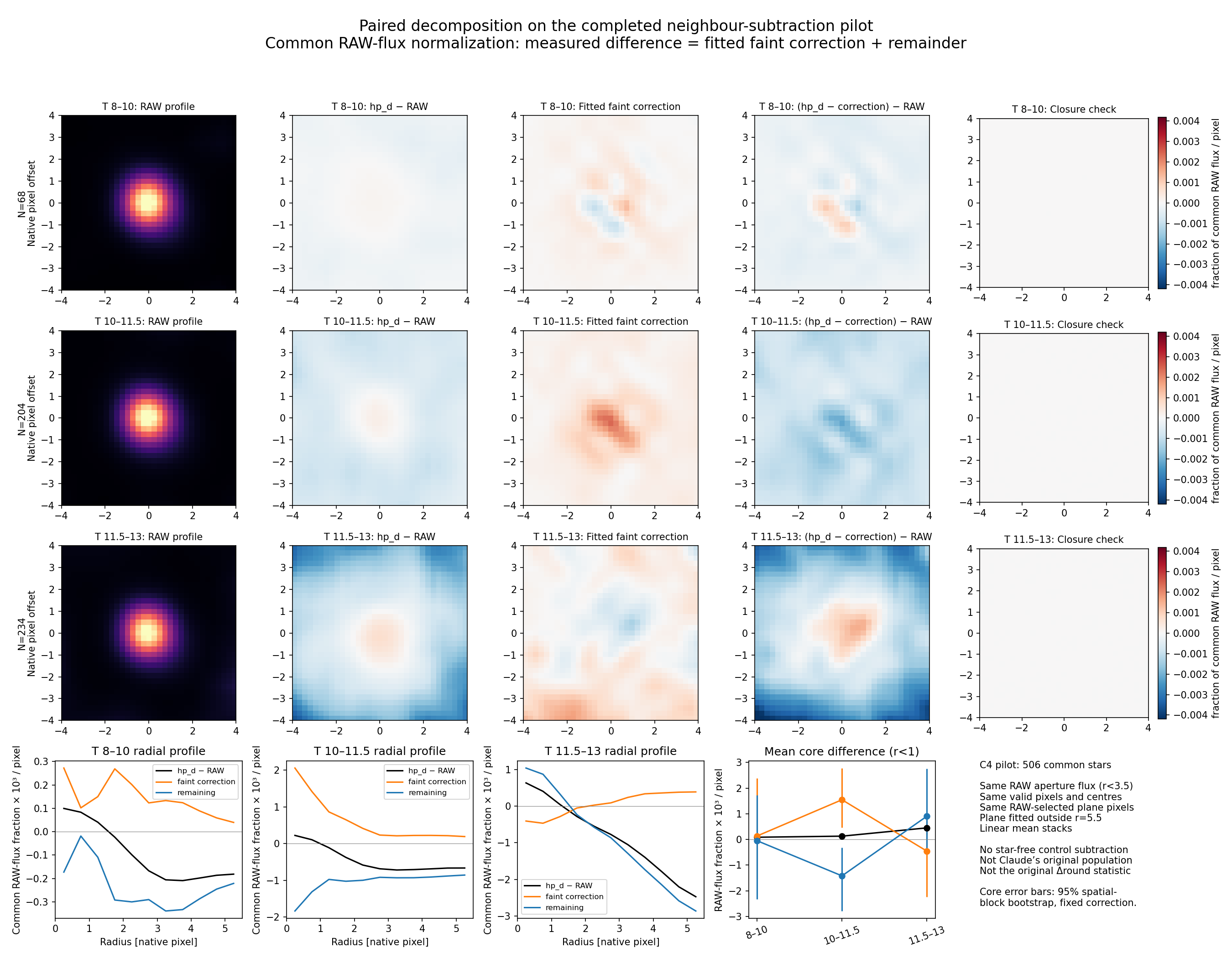
Rows are magnitude bins. Columns show the RAW profile, measured hp_d minus RAW, fitted faint correction, remaining difference after correction, and numerical closure. All difference images share a colour scale. The lower panels show radial profiles and mean core differences; error bars resample 128-pixel spatial blocks with the already fitted correction fixed. Those intervals do not include uncertainty from re-estimating the correction or the reference PSF.
This is deliberately labelled a companion plot, not a reproduction of Claude's result: the source population is the pilot's subset, there is no shifted star-free control subtraction, and the plotted scalar is a core difference rather than the historical Delta-round statistic. Raw data, planes, normalizations and component stacks are retained in analysis/paired_raw_decomposition.npz; tables/paired_raw_decomposition.json records the method and core summaries. Code: code/faintsub_paired_decomposition.py.
Conclusion of this plot: the fitted correction does not cleanly remove the measured RAW-to-hp_d pattern on this pilot sample. Its radial/morphological mismatch is visible. This does not refute the earlier expected light-budget scale or reproduce the original controlled shape statistic.