Targeted faint-star photometry
1,000 Gaia-associated sources selected at PS1-derived T=13–19. Nine patches across S24 / camera 2 / CCD 2. Two actual FFIs, 7.50 hours apart. Investigation started 2026-10-02.
Measurements · Image evidence · Validation · Data and reproducibility
Conclusion
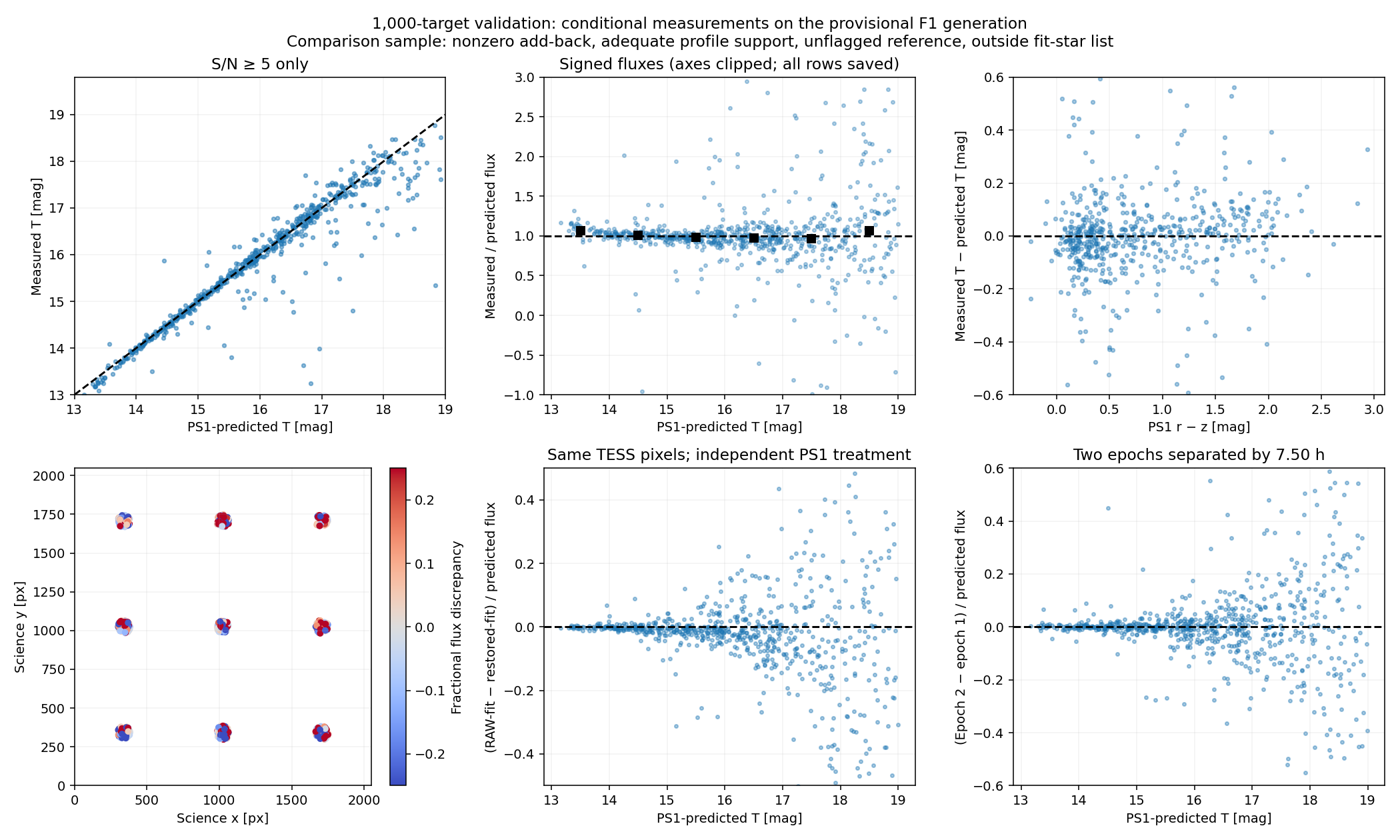
The actual per-band add-back and extraction procedure is implemented and has been exercised on all 1,000 targets. This is a separate endpoint test, not an inference from adding neighbours to the ePSF model. The packaged producer agrees with the reference transport to floating-point precision; measured fluxes broadly agree with PS1 predictions, with magnitude-dependent scatter and clear difficult cases.
Twenty targets have a zero transported component and are retained in the delivered measurements, but excluded from the primary add-back comparison. Thirteen targets fail because the target is masked or not independently identifiable. A numerical “ok” is not a scientific quality certificate.
Measured flux versus PS1 prediction
The table uses PS1 forced-mean fluxes as a reference and bins the unchanged sample by its stack-based selection magnitude. All signed TESS fluxes are retained. It additionally requires adequate profile support, a nonzero add-back, unflagged stack reference inputs and forced-mean predicted-magnitude uncertainty below 0.1 mag. The first real epoch is shown; both epochs and every excluded/failed row are downloadable.
| Selection T | N | Median flux offset | Statistical 95% interval | Robust scatter | Median S/N | Nonpositive |
|---|---|---|---|---|---|---|
| 13–14 | 46 | +1.0% | [+0.1, +2.6]% | 4.6% | 212.0 | 0 |
| 14–15 | 115 | +0.1% | [-0.3, +0.9]% | 3.1% | 115.4 | 1 |
| 15–16 | 157 | -1.7% | [-2.7, -1.0]% | 5.1% | 45.8 | 0 |
| 16–17 | 173 | -2.4% | [-4.1, -0.1]% | 12.2% | 17.1 | 5 |
| 17–18 | 139 | -3.0% | [-8.4, +1.0]% | 25.4% | 7.7 | 7 |
| 18–19 | 129 | +6.7% | [-0.4, +18.4]% | 58.2% | 3.7 | 14 |
Offsets are 100 × (median measured/predicted flux − 1). Scatter is 1.4826 × MAD of that ratio. Intervals resample stars and do not include shared calibration or template systematics. Magnitudes of low-S/N detections are biased by positivity selection; they are not used to infer faint-bin agreement.
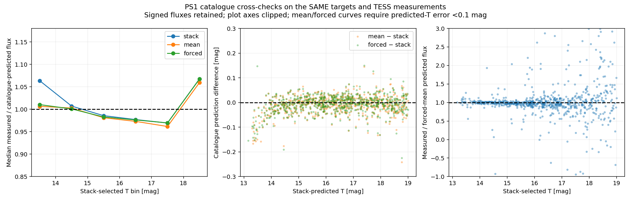
The catalogue choice accounts for most of the apparent bright-bin offset against stack photometry. PS1’s guidance notes that mean PSF photometry is less noisy for bright objects but becomes detection-biased near the single-epoch limit, whereas forced-mean measurements include all warps. Bright-end saturation and imperfect stack PSFs remain reference limitations. The forced-mean fluxes are in Jy; all catalogue variants use the same adopted band mix and fixed conversion.
Aperture cross-check
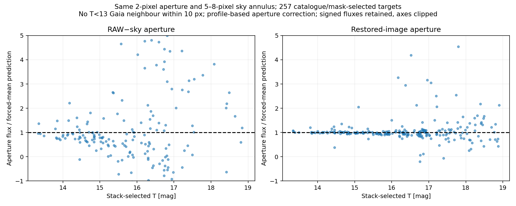
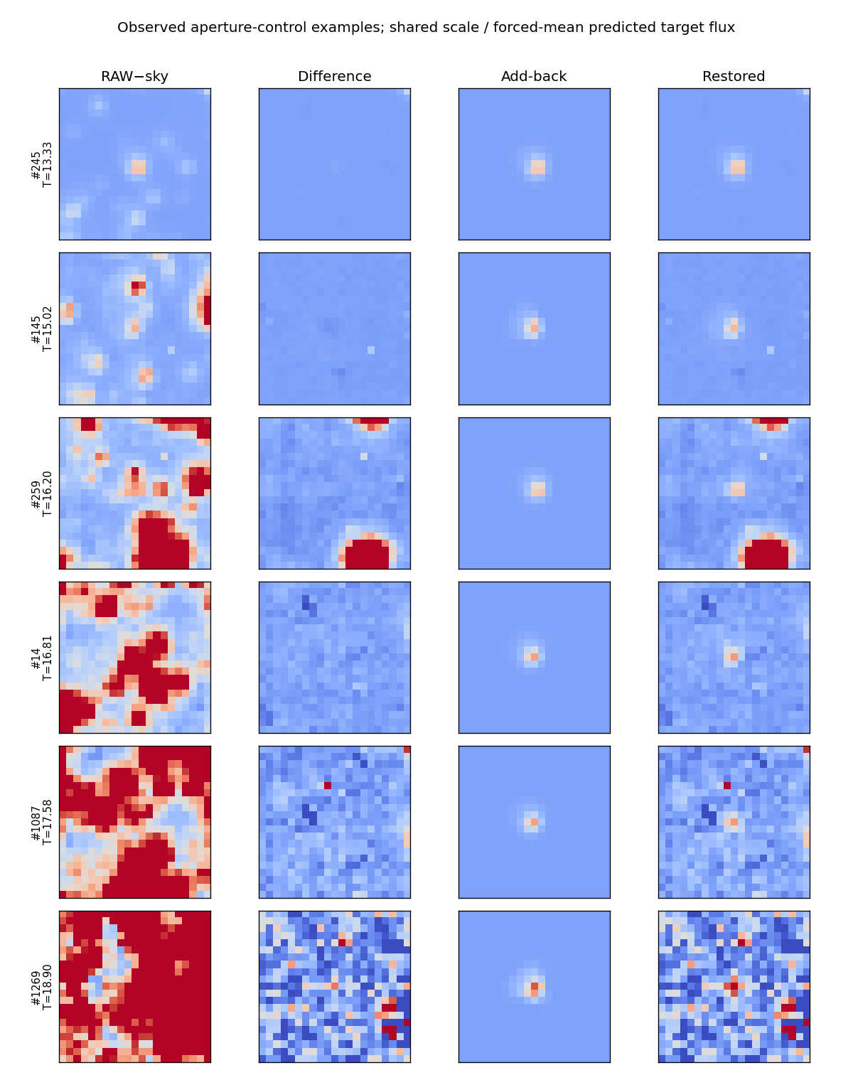
On a catalogue/mask-selected subset of 257 targets with no Gaia T<13 neighbour within 10 pixels, the same 2-pixel aperture and 5–8-pixel sky annulus were measured before and after de-crowding. Median absolute fractional discrepancy against forced-mean prediction is 143.8% for RAW and 8.1% after restoration. This subset result is not an all-crowding guarantee; both use the same model-based aperture correction.
Sample and a corrected selection error
The first attempt cross-matched against the production Gaia catalogue, whose metadata has magnitude_limit: 18.0. It therefore could not represent T=18–19 and biased its few objects near the limit. That cohort is superseded. A private Gaia DR3 G<22 query, without a T cut, supplies the final selection and nuisance catalogue. All original T≥17 objects and all reference-fit participants were replaced using catalogue information alone. No measured TESS flux was used for selection.
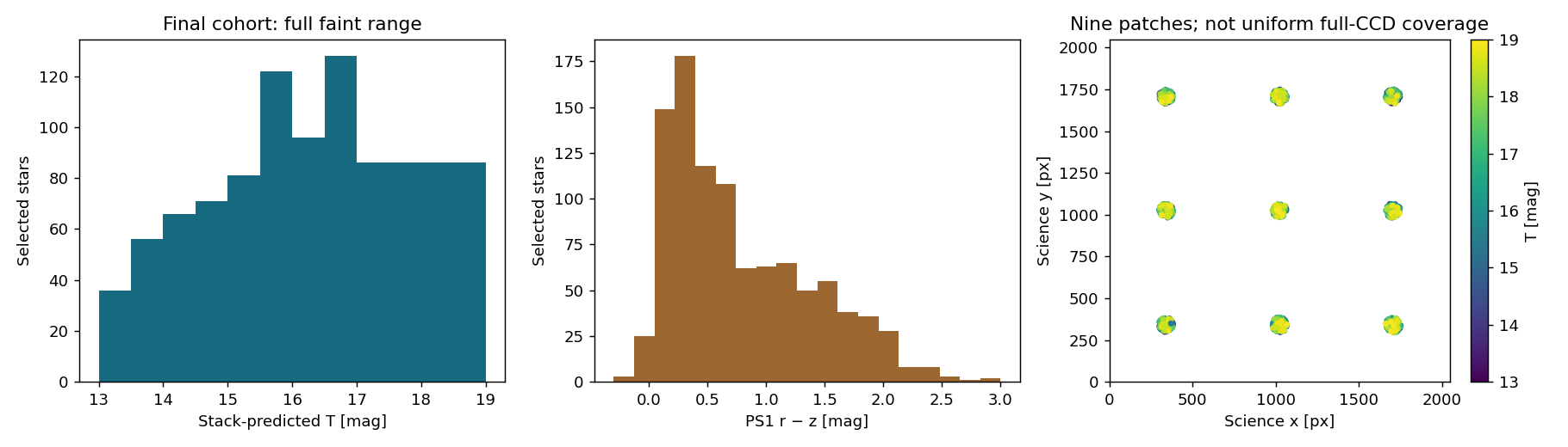
The final range is 13.122–18.999, including 86 stars in each half-magnitude bin from 17 to 19. No final target appears in the reference-fit source list. This is not a K-fold pixel-held-out ePSF experiment. The nine sky patches sample position but do not establish behaviour at every CCD edge or optical-axis location.
Subpixel-phase-aware stacks (2026-10-03)
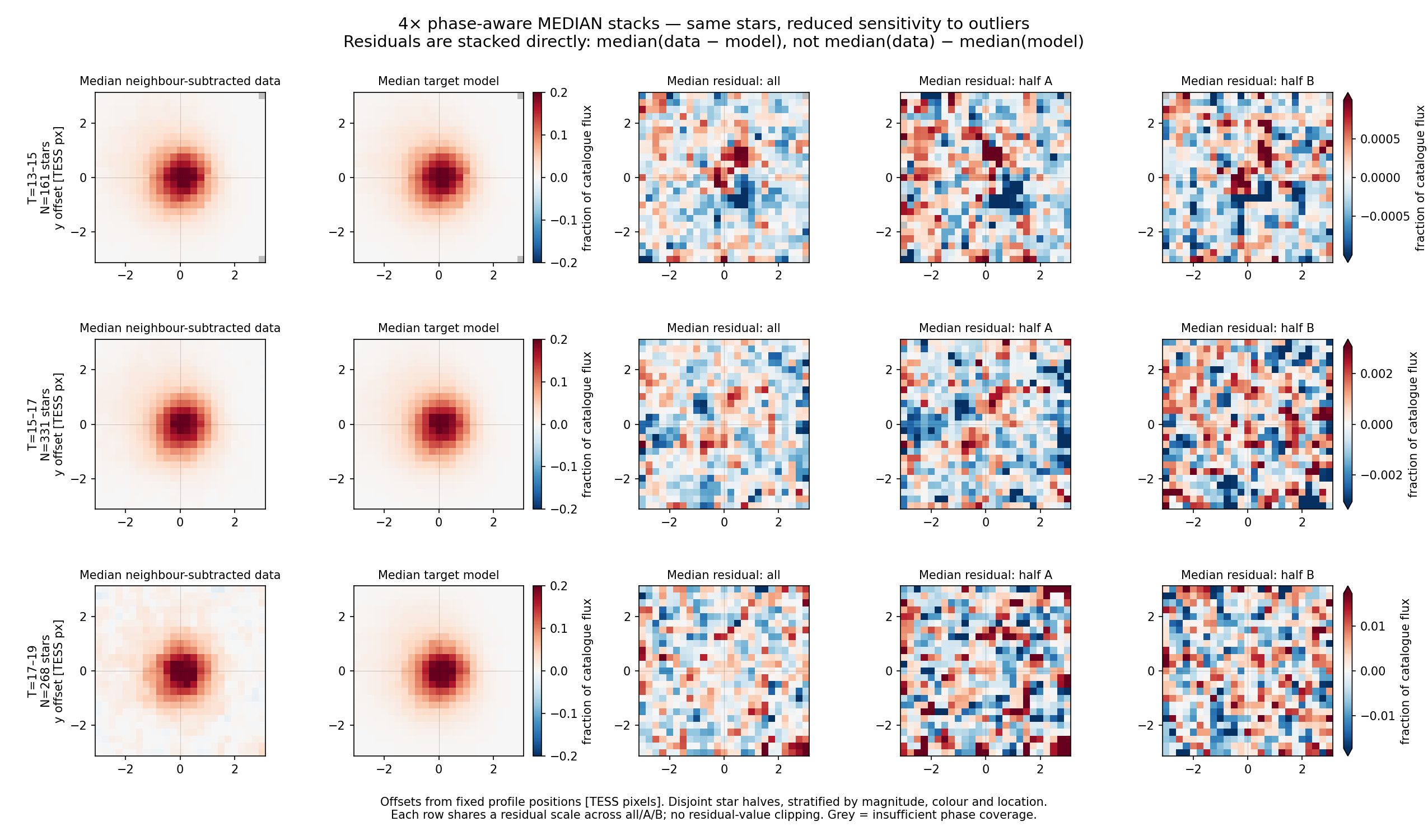
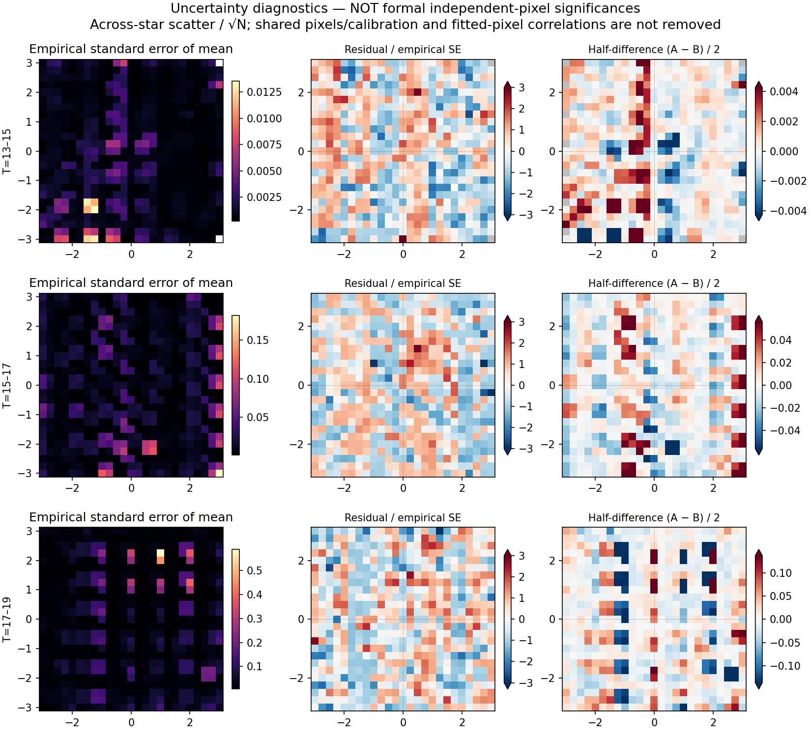
Conclusion: the registered median stack exposes a weak central positive/negative pattern in the brighter group. Agreement between disjoint star halves is modest, and residual amplitudes are comparable to empirical uncertainty. This is a tentative structure, not a secure ePSF-error detection. The faintest stack has no clear repeating pattern. The un-clipped mean is strongly sensitive to large individual residuals. Neither result establishes pure Poisson noise or a universal absence of structural error.
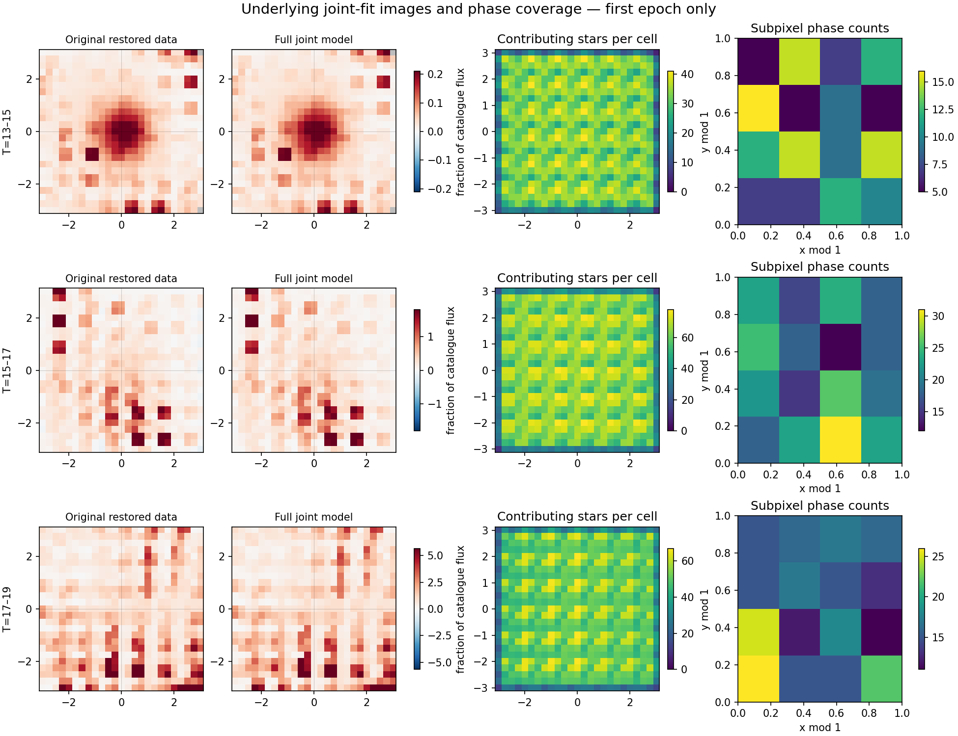
The unchanged first-epoch comparison sample contains 161 stars at T13–15, 331 at T15–17, and 268 at T17–19. Positions and masks are frozen. Native pixel samples are placed on a 4× grid (0.25 TESS pixel spacing), using the existing bilinear rasterizer. The output spans ±3 pixels. No centring on residual peaks, refitting, or residual-value clipping was done. Both mean and median estimates are shown.
Method and denominators
$$r_{s,p}=(D_{s,p}-M_{s,p})/F_s,$$Here $s$ labels a star and $p$ a native pixel; $D$ is its restored observation, $M$ the full fitted joint model, and $F_s$ the fixed PS1-predicted total stellar flux. All three are in electrons per second, so $r$ is dimensionless. Each pixel is registered at its offset from the saved fractional-pixel stellar position. The rasterizer accumulates bilinear numerator and coverage weights; their ratio gives each star's raster value. Samples with coverage weight below 0.05 are missing, not zeros.
For the isolated-image panels, the fitted nuisance contribution is subtracted from the observation; the target model is the fitted target amplitude times its existing profile. Their difference is exactly the original joint residual. The median residual is calculated directly from per-star residuals; it is not the difference of independently computed median data and model. The mean gives every contributing star equal weight at each grid location. At least eight contributors are required for a full-stack pixel, four for a half-stack pixel.
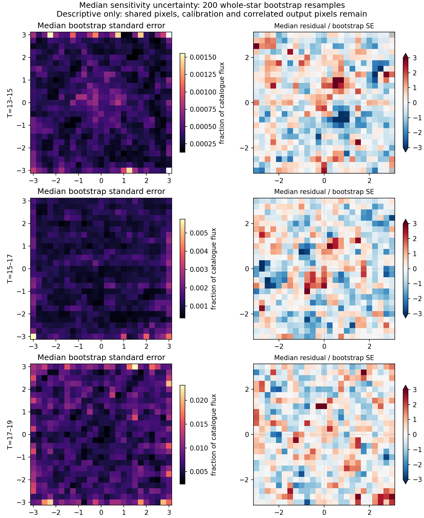
The two disjoint star halves use a fixed seed and stratification by magnitude, colour and CCD location. They share the original FFI/calibration, and nearby stamps can share pixels; they are therefore not fully independent noise realizations. The median uncertainty uses 200 whole-star bootstrap resamples. The mean uncertainty is across-star scatter divided by the square root of the contributing count. Neither corrects shared-source/FFI covariance, model uncertainty or the variance reduction from fitting those same pixels.
Amplitude and uncertainty within 2 pixels of the target
| T range | Median-map RMS | Median bootstrap SE | Half-map correlation |
|---|---|---|---|
| 13–15 | 0.050% | 0.039% | 0.23 |
| 15–17 | 0.106% | 0.097% | 0.16 |
| 17–19 | 0.548% | 0.571% | −0.11 |
Percentages refer to catalogue total flux per sampled native-pixel amplitude. RMS is a descriptive map amplitude, not a bias in total flux; bootstrap SE varies across the map. The ratio of these table columns is not a global significance. Half-map correlations are descriptive, with correlated output cells.
Un-clipped mean and half-difference checks
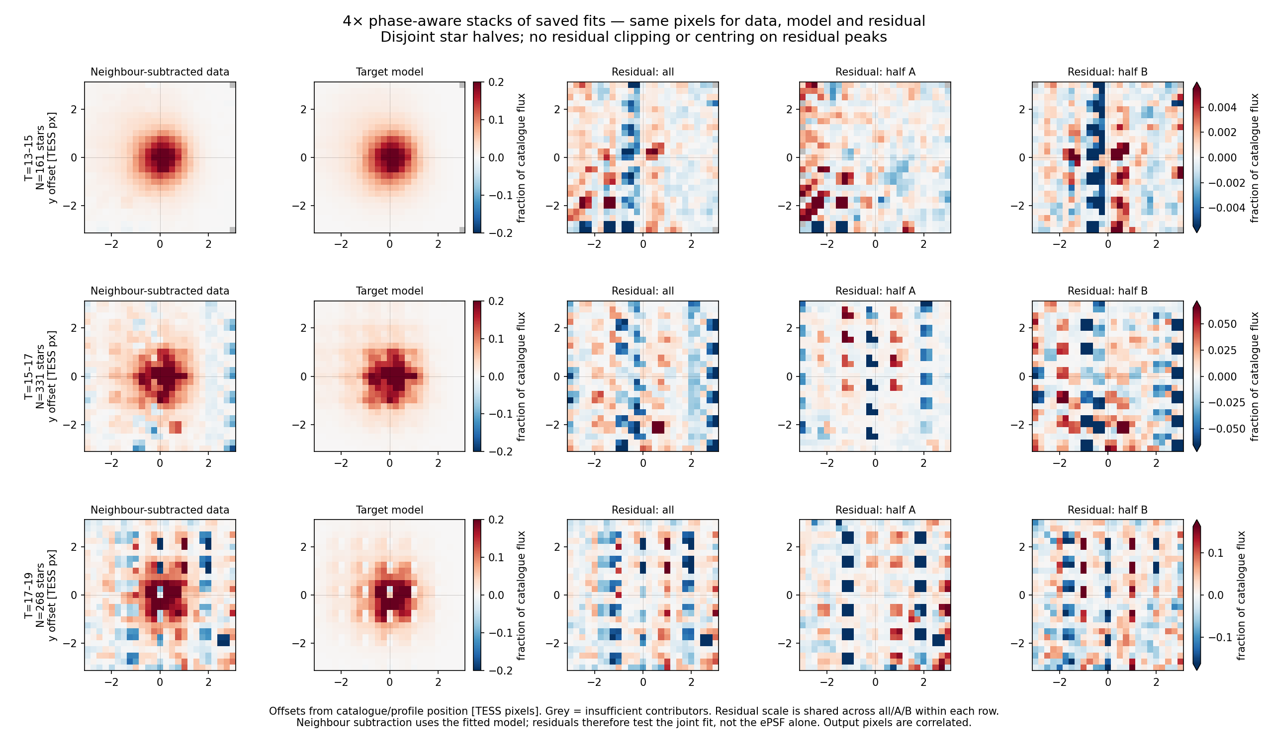
Original observations, joint models and phase coverage
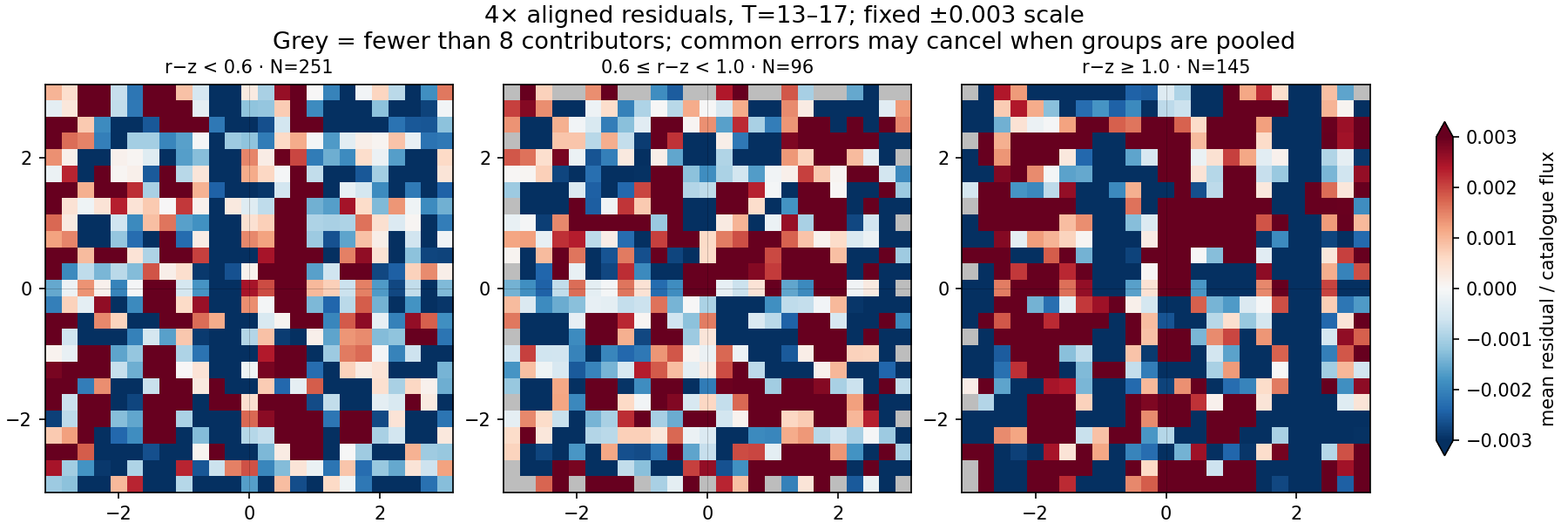
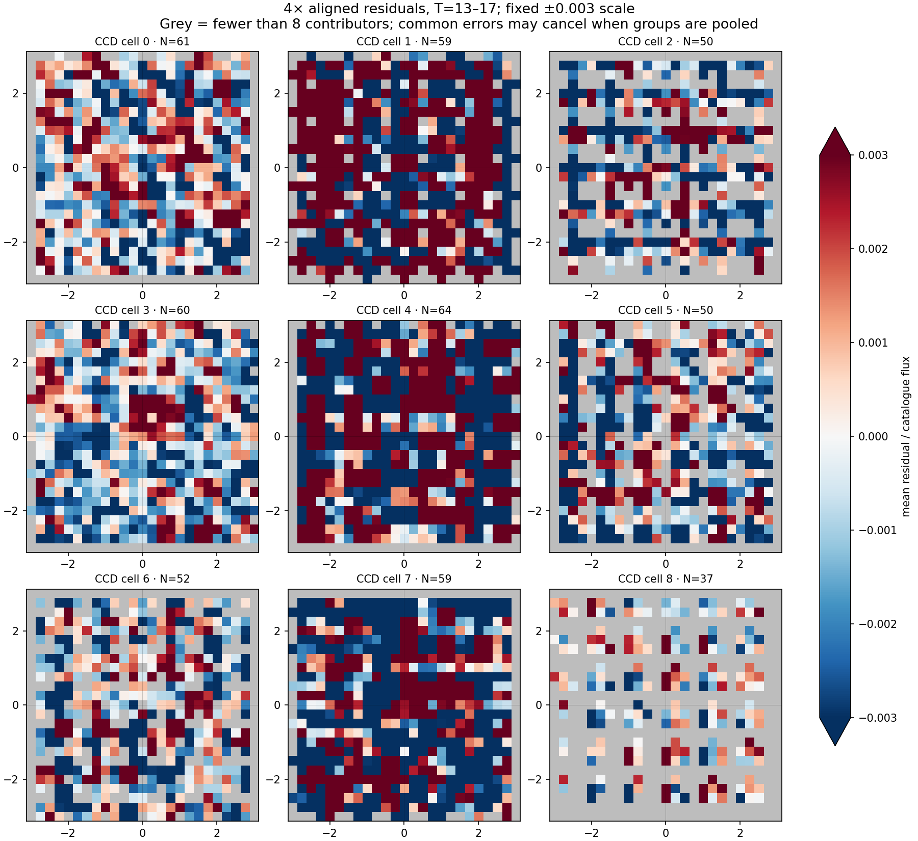
Colour and detector-position splits
Un-clipped means for T13–17, at the same ±0.003 scale (±0.3% of catalogue flux). Many values clip, and several small spatial groups lack adequate phase coverage. These views expose heterogeneity; they cannot establish absence of colour/spatial effects.
Validation and reproducibility
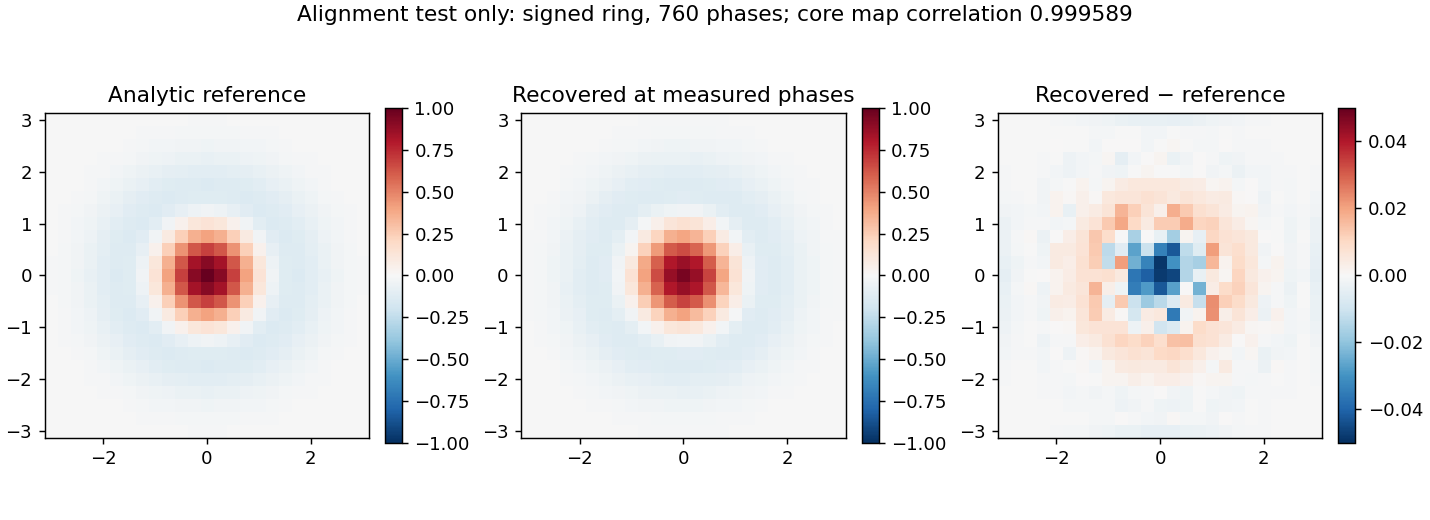
Coordinate checks verify constant preservation, all-masked output, and the exact fractional displacement of an impulse. An analytic signed ring sampled at the actual stellar phases is recovered with map correlation 0.9996, verifying alignment only. Data minus model equals the independently rasterized residual to numerical precision. Oversampling does not deconvolve the native pixel response or create independent information.
Record · Input hashes and method · Source IDs and half assignments · Stack arrays and uncertainties · Per-star raster arrays · Generator
Conclusion: weak bright-star structure is worth following up, but its current reproducibility and uncertainty do not justify claiming either a detected common ePSF defect or purely Poisson residuals. A larger independent-star sample and a fitted-noise null would be needed to decide that.
Residuals relative to the input noise
See the stellar centre directly
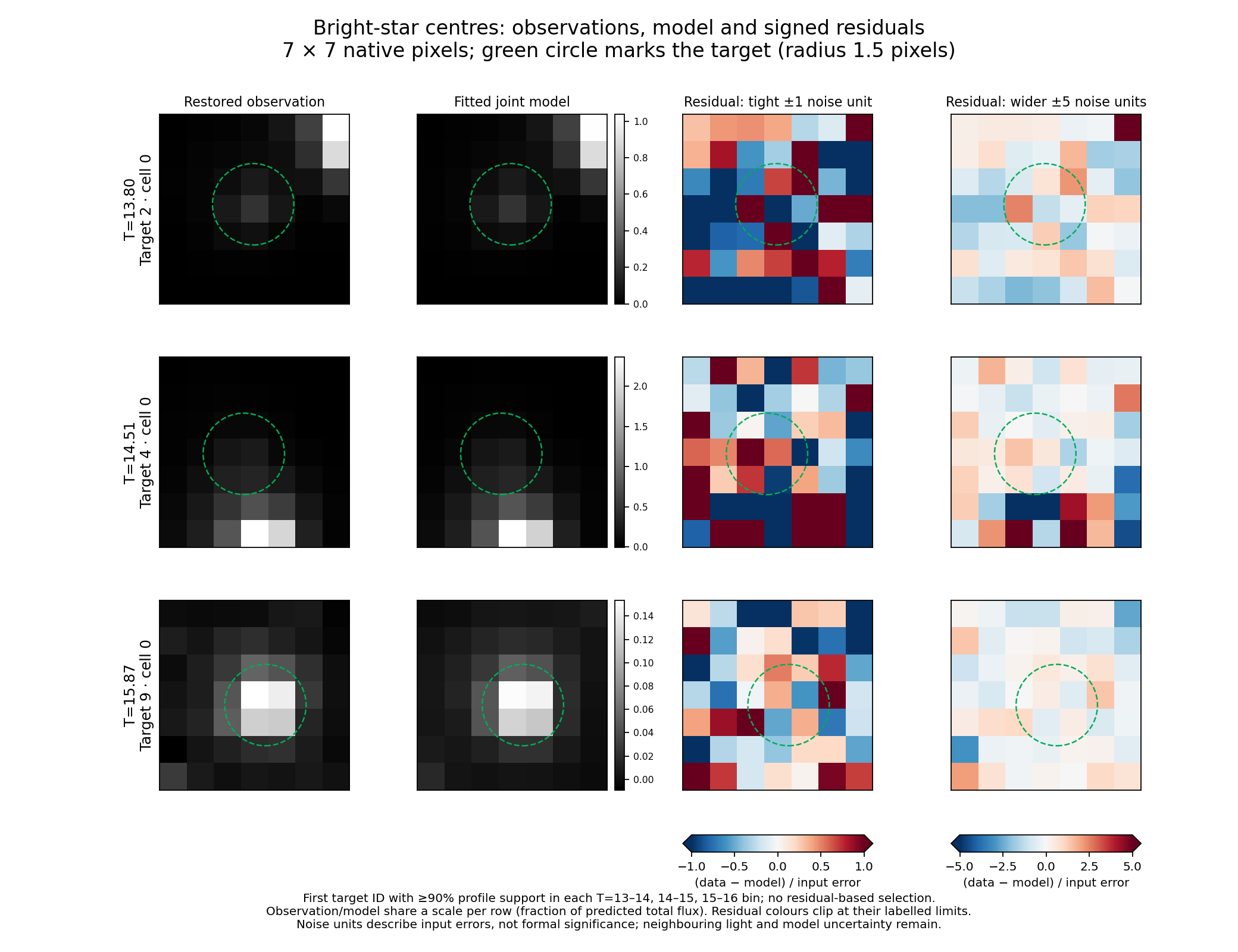
Updated 2026-10-03: enlarged 7×7-pixel examples with the target circled. The third column uses a tight signed −1 to +1 input-error scale; the fourth shows the identical residual at −5 to +5. Red means excess observed light, blue means excess model light, and white is zero. Endpoint colours are clipped, so use the wider view to judge amplitude. Targets are the first eligible IDs with at least 90% profile support in each bright magnitude bin, not chosen by residual appearance. These examples locate the residual; they do not establish a universal ePSF error pattern.
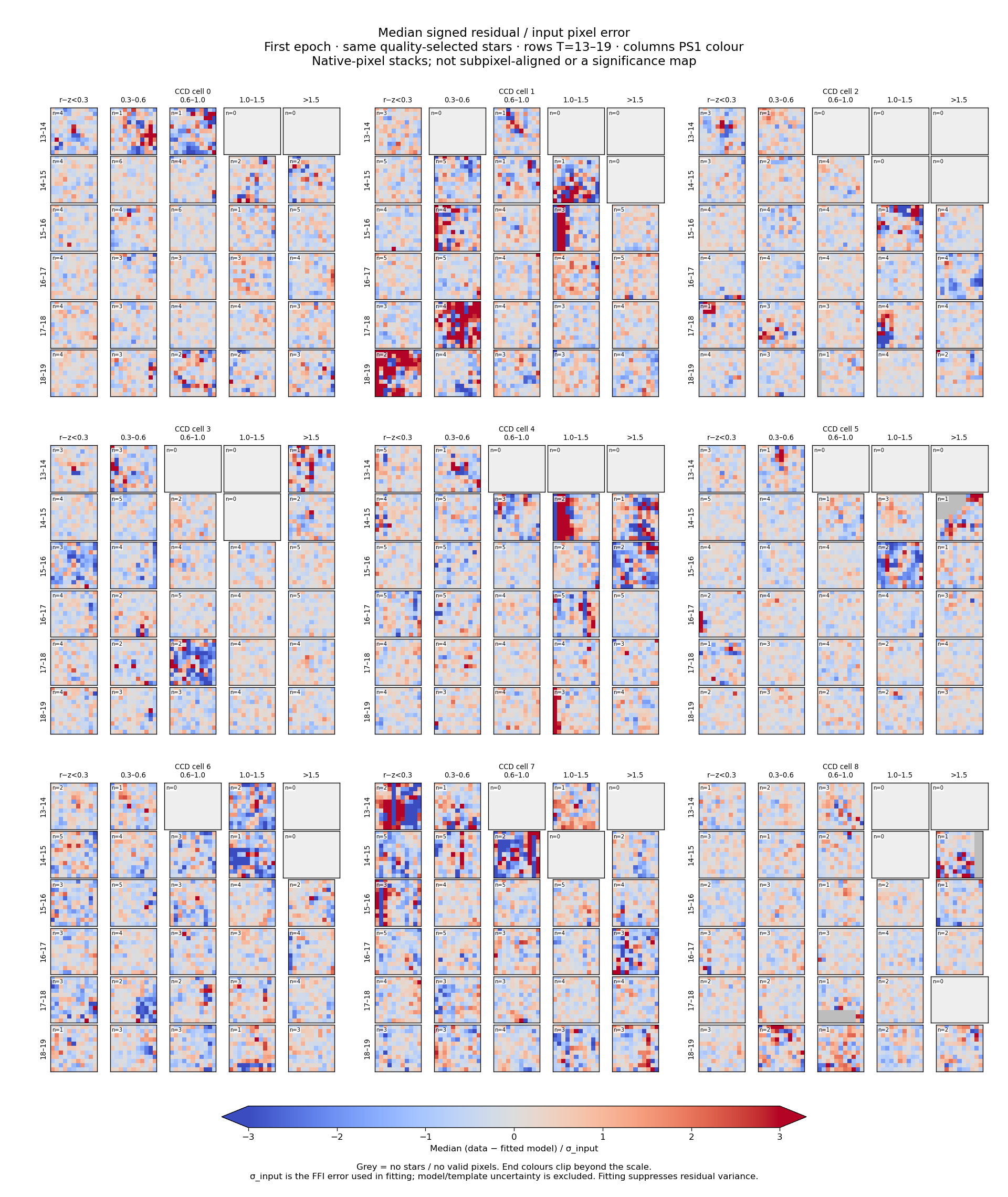
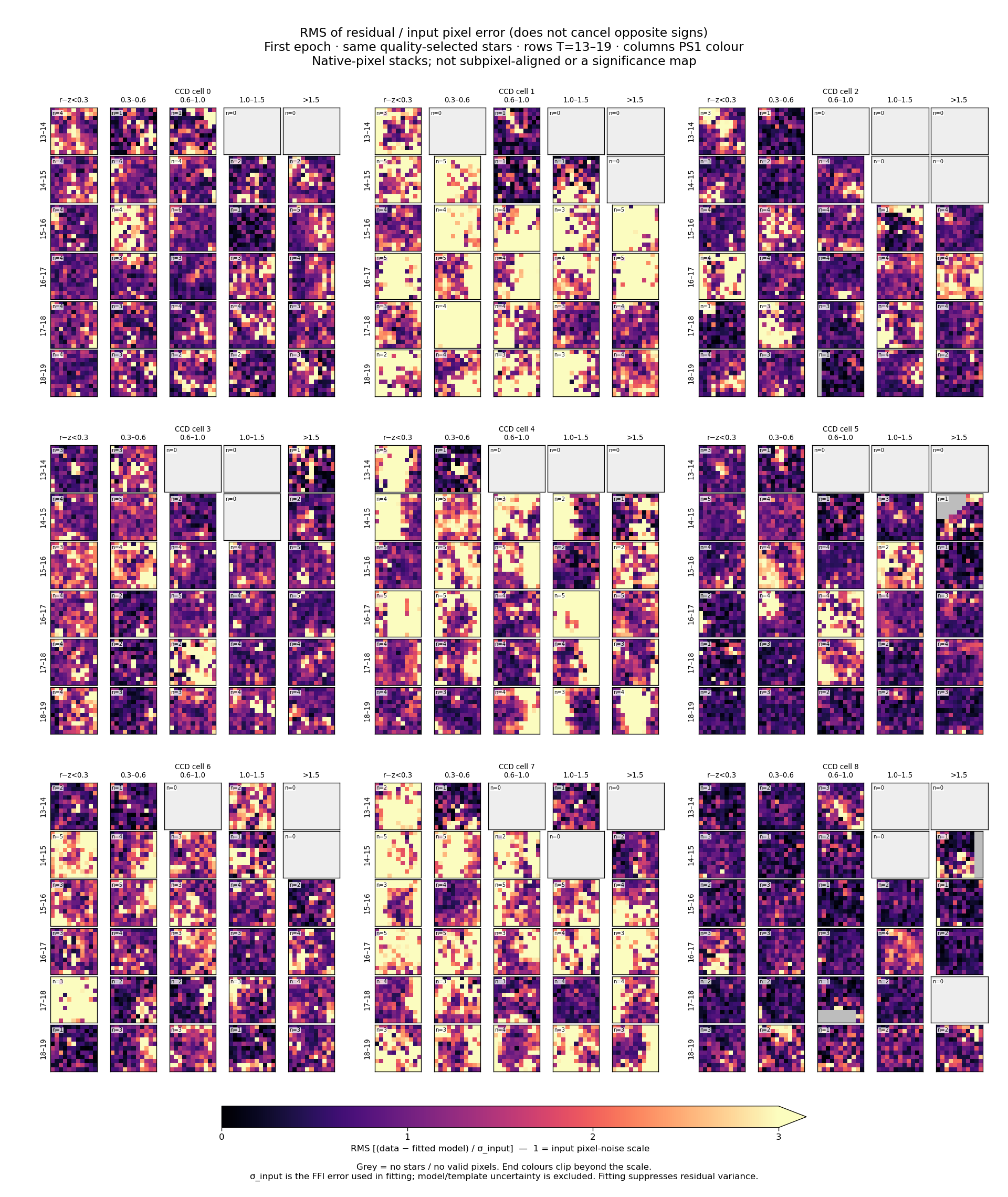
Added 2026-10-03 to reveal residuals hidden by the fractional-flux scale. The same first-epoch comparison sample and masks are used. Each residual pixel is divided by the original FFI error used in the fit:
$$z_{s,p}=\frac{D_{s,p}-M_{s,p}}{\sigma_{s,p}}.$$Here $s$ identifies a star and $p$ a native stamp pixel; $D$ is the restored observation, $M$ the fitted joint model, and $\sigma$ the input FFI pixel error, all in electrons per second. The ratio $z$ is dimensionless. Panels show either the median of $z$ over stars or its root mean square. No subpixel alignment or refitting is performed.
Inspection conclusion: some bright-star bins show residual amplitudes above the input pixel-noise scale, hidden by the previous fractional-flux display. Small fractional residuals therefore do not establish noise-limited fits. These sparse-bin views do not isolate ePSF error from neighbour/background residuals or noise-model errors.
Read the labelled colour bars: the signed median spans −3 to +3 input-error units; the RMS spans 0 to 3, with 1 marking the input pixel-noise scale. End colours clip larger values. RMS exposes discrepancies that cancel in a signed median. These are not formal significance maps: fitting the same pixels suppresses residual variance, noise/model correlations are not corrected, and template/ePSF/calibration uncertainty is excluded. Each bin still contains few stars.
Underlying images
Each grid uses the same colour × magnitude × 3×3-position groups. Stars are normalized by the stack-based catalogue prediction solely for display. No S/N cut is imposed on these stacks. Counts can be small; grey panels have no eligible sources. Faint groups visibly contain large fluctuations and neighbouring-source residuals, so the aggregate comparison must not be read as precision photometry for every target.
Restored observations and actual transported light
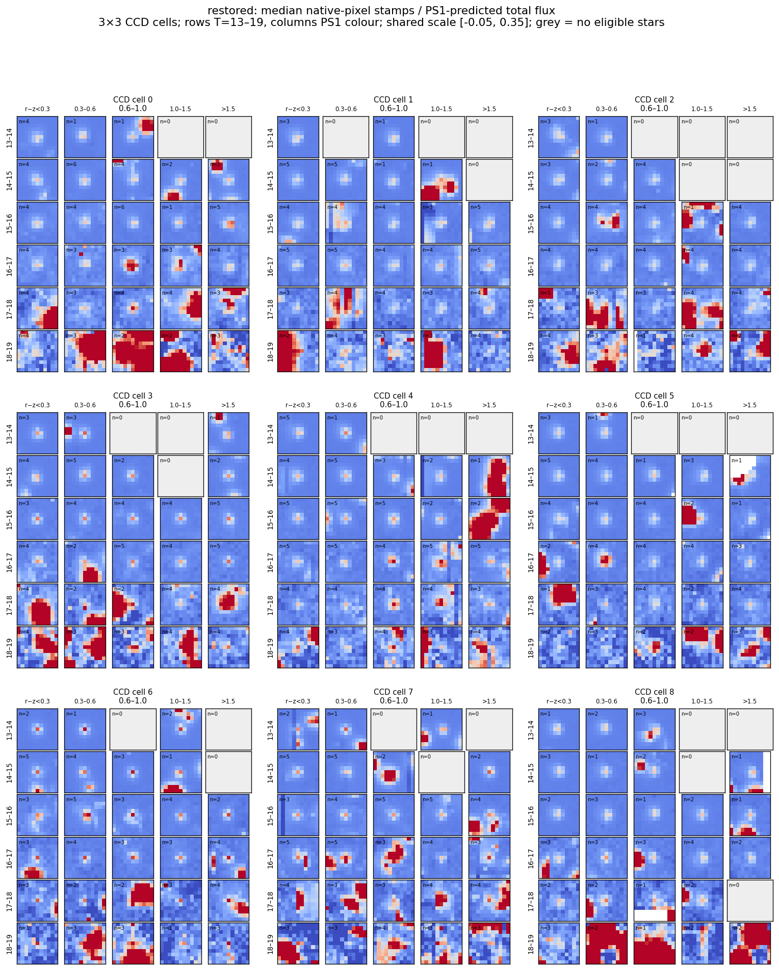
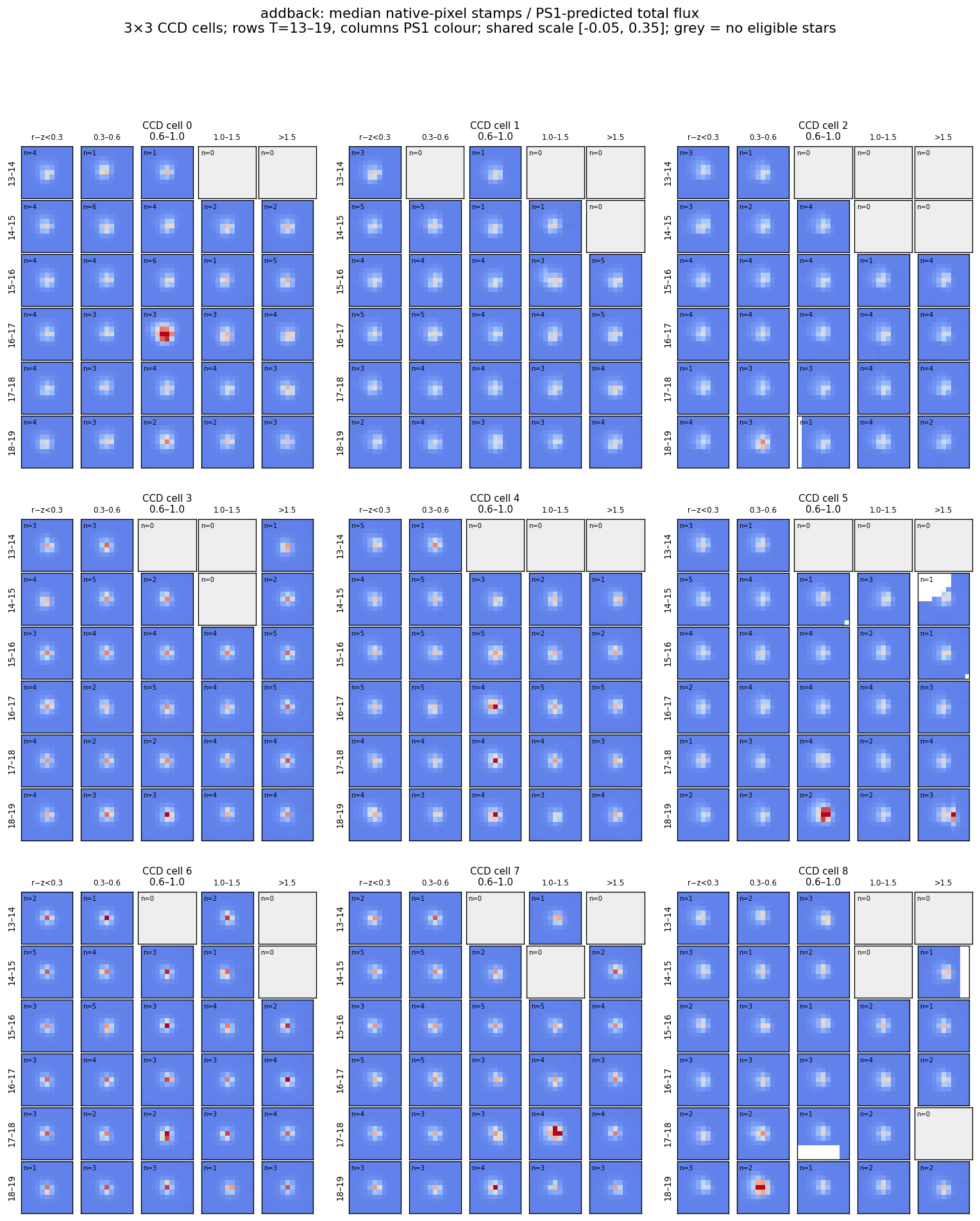
Residual stacks and RAW-image control
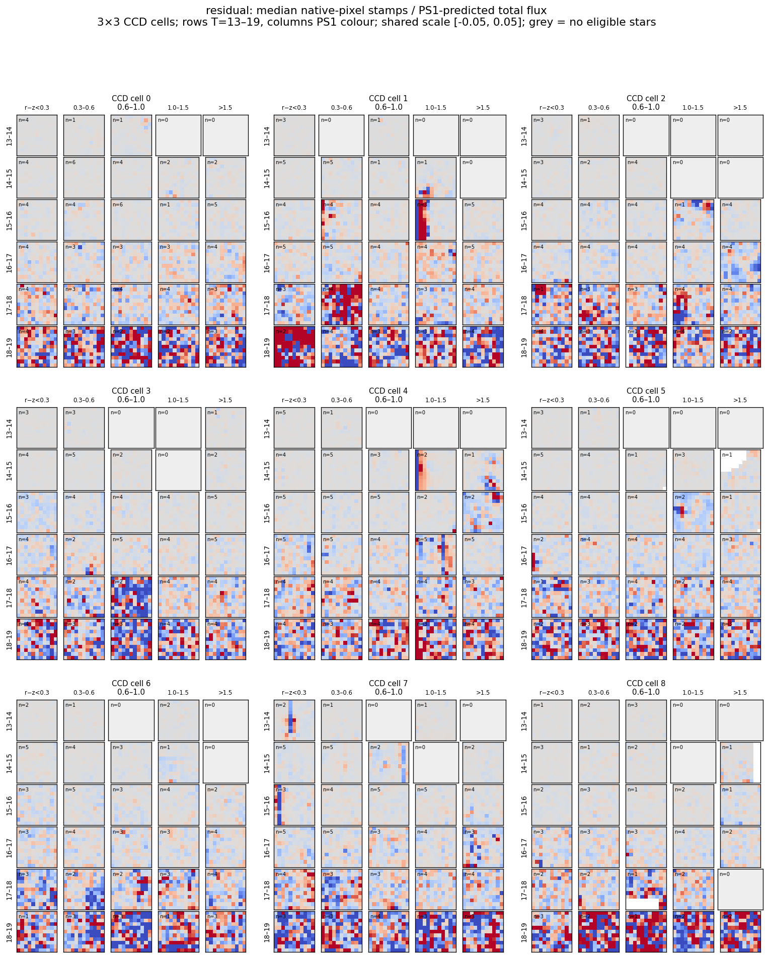
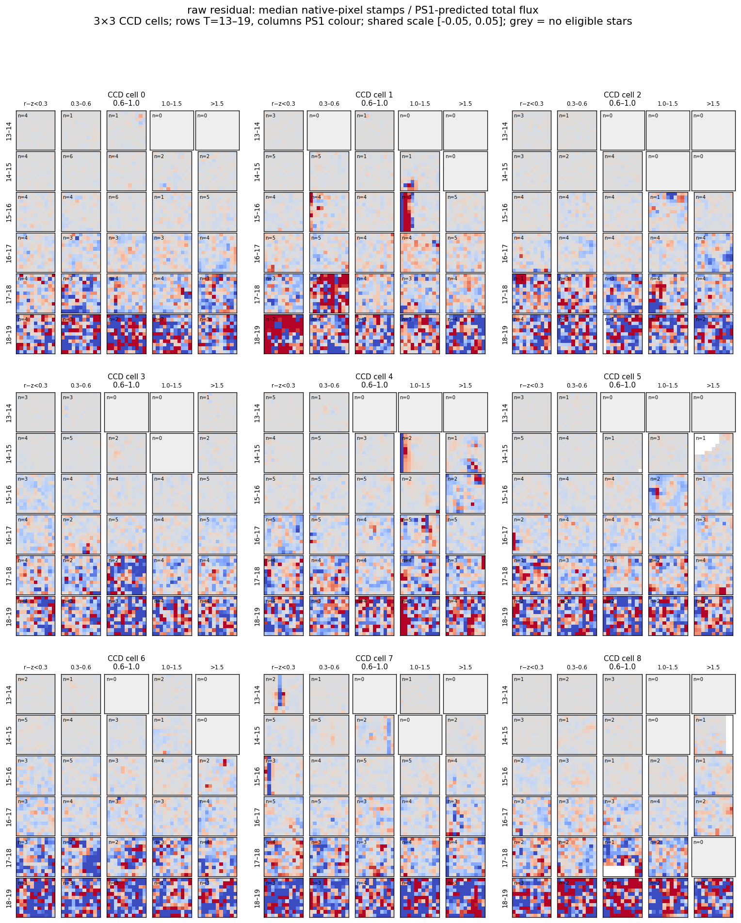
The RAW control uses the same TESS pixels and PSF basis without PS1 subtraction/add-back. Its noise is correlated with the restored estimate; their difference is a diagnostic, not an independent-error significance test.
Individual observed, model and residual stamps
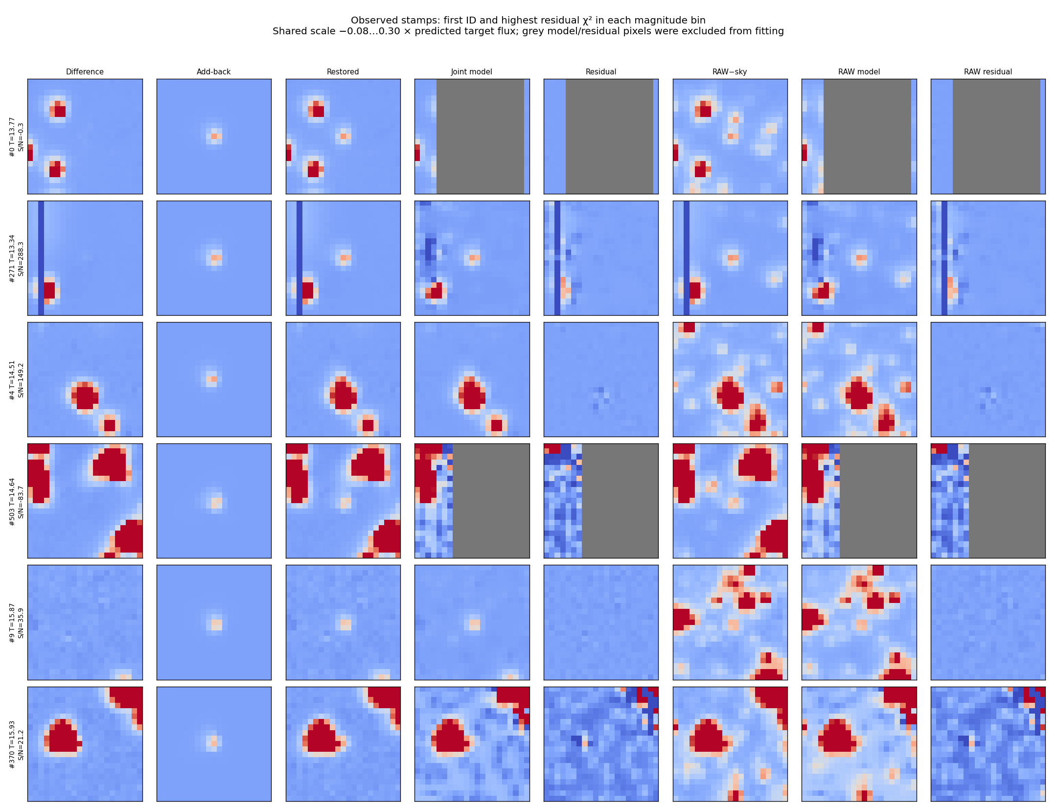
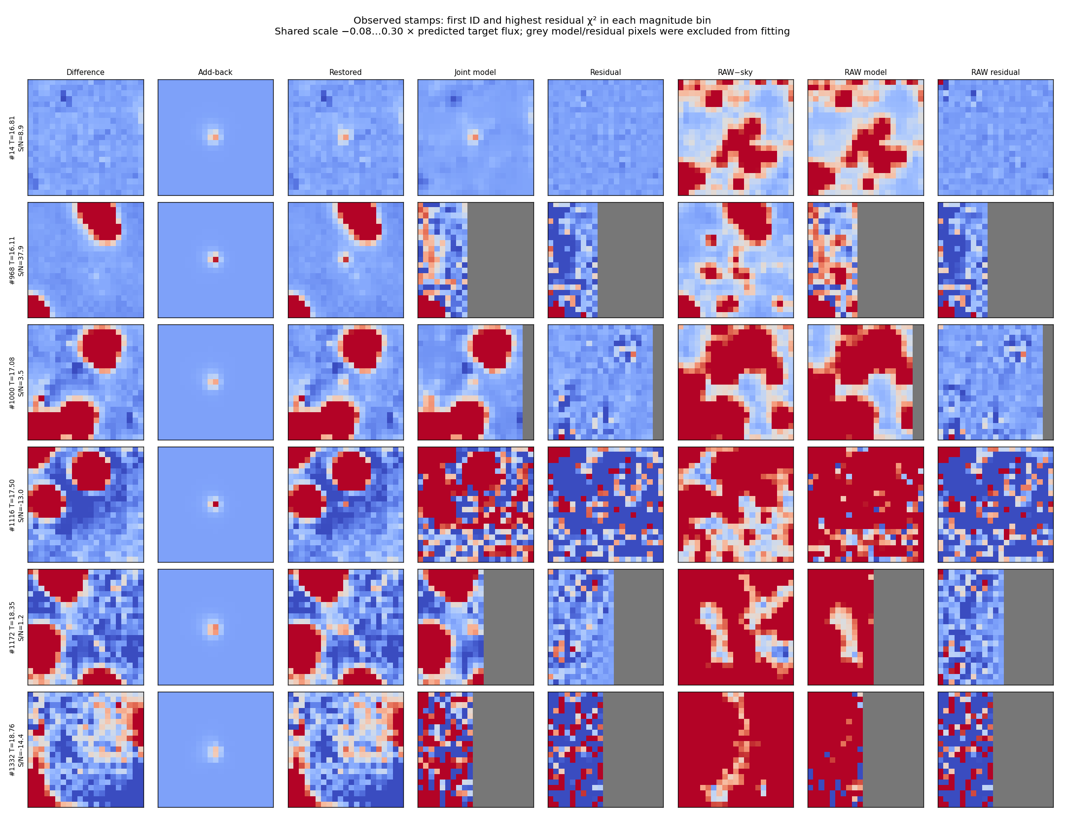
All failed targets
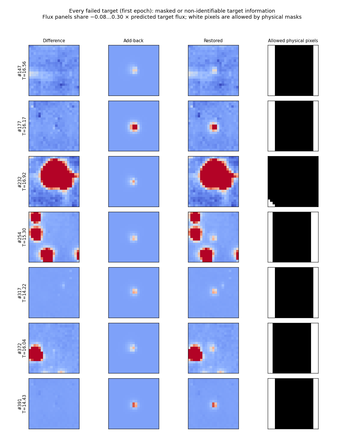
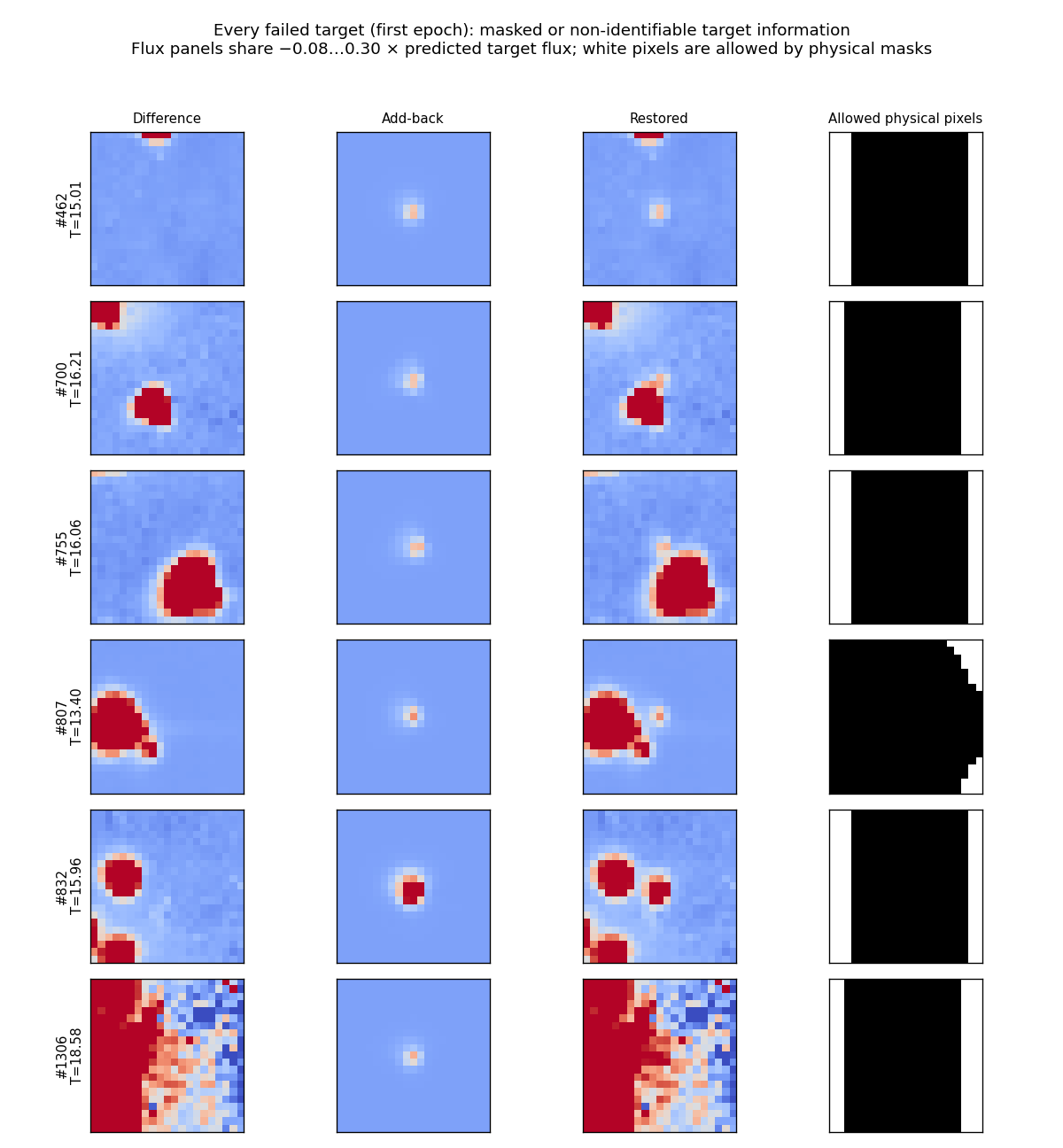
What was tested
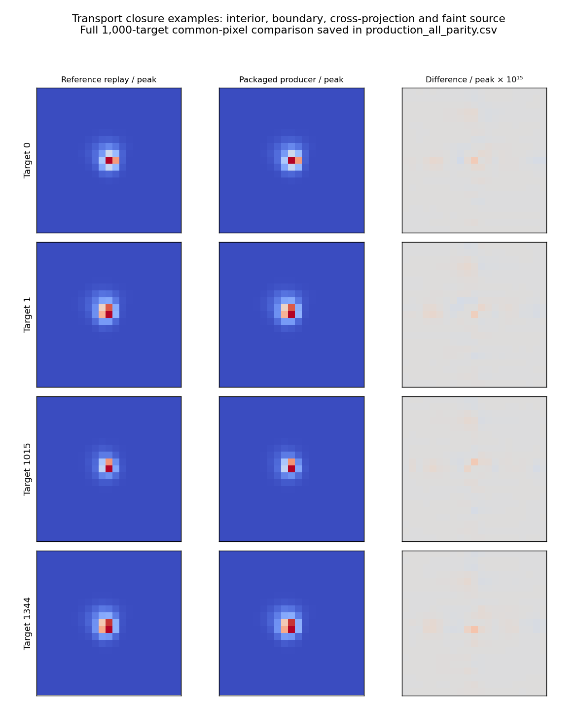
- Operator reproduction: all 1,000 packaged components agree with the validated replay on common pixels; maximum relative L2 difference is 4.94e-16. Twenty-four windows use a different centre, so the comparison explicitly aligns their global coordinates.
- With/without-source blur closure: 524 diagnostic interior cases reach maximum relative L2 2.86×10⁻⁶, below the 10⁻⁴ target-flux tolerance. Production/reference parity and this finite-precision subtraction test are different checks.
- Signed photometry: negative fluxes, masked cores, duplicate nuisance columns and per-frame component/zero-point changes are covered by tests. The target flux is not fixed to a catalogue prior.
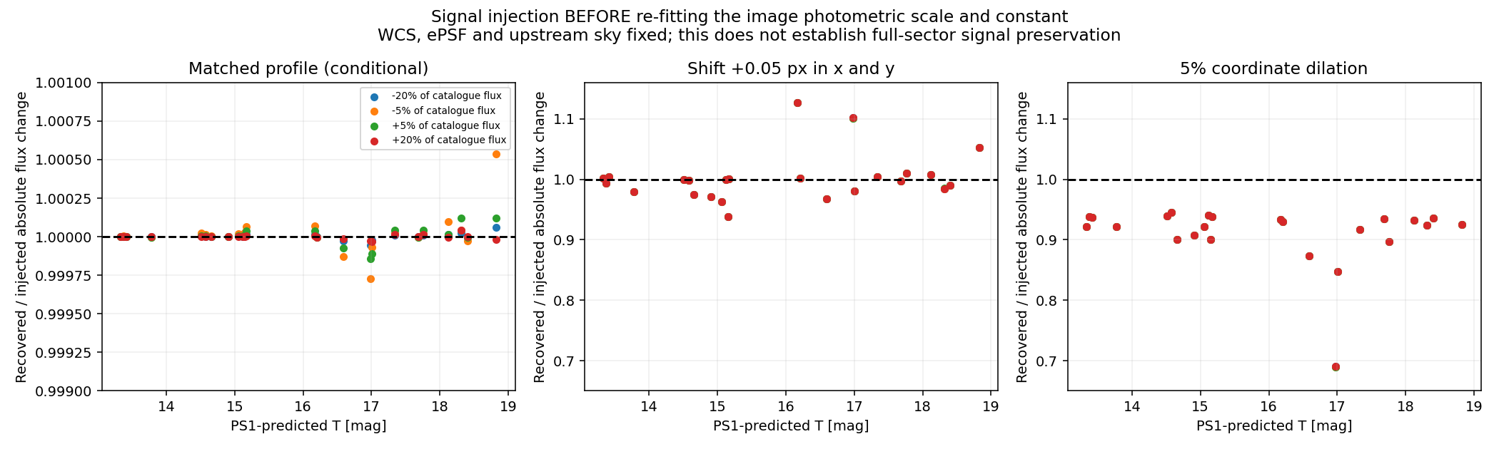
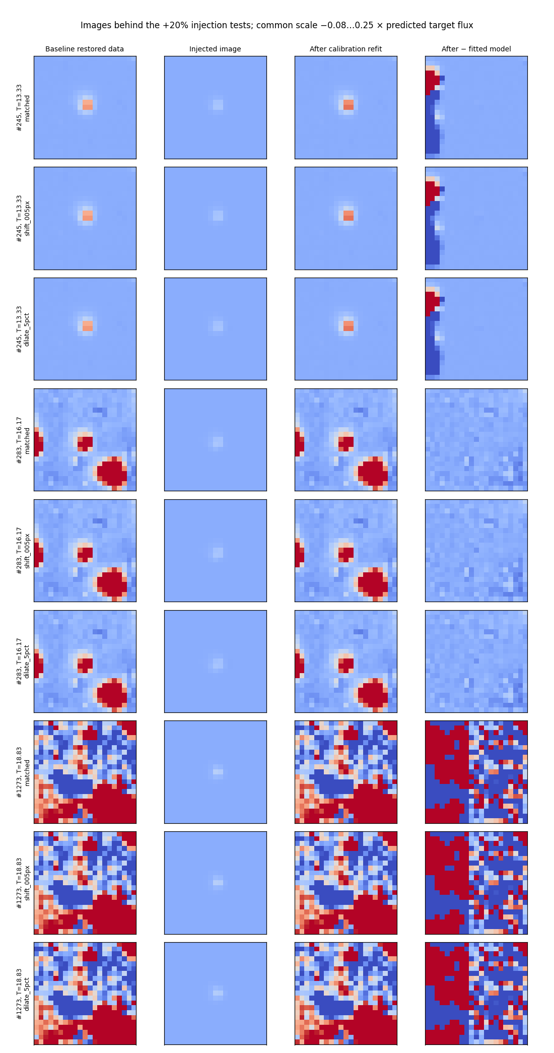
- Signal response: 24 stars × four signed amplitudes per profile scenario, injected before re-fitting the image scale and constant. The matched-profile absolute-flux gain is within 0.054% of unity. It is a conditional test, not an independent PSF validation or a normalized transit-depth test.
- Model sensitivity: a 0.05-pixel shift and a 5% profile-coordinate dilation produce appreciable biases, especially in difficult cases. These are deliberate stress scenarios, not estimates of the real PSF error.
Actual injected images and fit residuals
Two-epoch repeatability
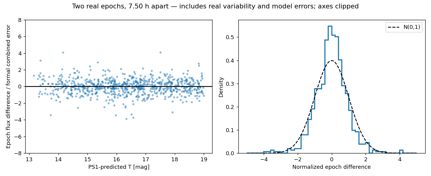
The real epoch comparison includes stellar variability and model error; no detrending was applied. Static errors can cancel between these two measurements, so short-baseline repeatability does not certify absolute fluxes or long-term signal preservation.
Method and normalization
For a target $t$, the restored image is
$$D_t(p)=D(p)+a(p)\sum_{b\in\{r,i,z,y\}}\mathcal L_b[S_{t,b}](p).$$$p$ is a native science pixel; $D$ and $D_t$ are difference/restored intensities in electrons s$^{-1}$ per pixel. $S_{t,b}$ is the retained target component in band $b$, in the stored PS1 linear-rate units per PS1 pixel. $\mathcal L_b$ replays the producing blur, ownership/padding, registration, band rescaling and source-position kernel interpolation. Its output uses native template flux units. $a$ is the saved fitted conversion to TESS electrons s$^{-1}$, evaluated at each output pixel. The subtraction’s constant is already in $D$ and is not added again.
$$D_t(p)=f_tP_t(p)+\sum_j f_jP_j(p)+\beta.$$$f_t$ is the fitted target flux in electrons s$^{-1}$. $P_t$ and $P_j$ are dimensionless pixel fractions of the frozen target/neighbour profiles, normalized on their complete represented support before masking or cropping. The $f_j$ are freely fitted neighbour residual amplitudes in electrons s$^{-1}$; they are not necessarily total stellar fluxes. $\beta$ is a fitted constant in electrons s$^{-1}$ per pixel. Weights come from raw FFI pixel uncertainties. Target-identifiability is checked after projecting out the nuisance column space.
$$T_{\rm PS1}=-2.5\log_{10}\!\left(\sum_b w_b10^{-0.4m_b}\right)+\Delta.$$$m_b$ are PS1 AB PSF magnitudes; $w_b=(0.254,0.4368,0.1654,0.1438)$ for $r,i,z,y$ are the adopted fixed weights. $\Delta=-0.305636$ mag is fixed from separate bright Gaia-XP synthetic photometry. For forced-mean data, replace $10^{-0.4m_b}$ by $F_b/(3631\,\mathrm{Jy})$, where $F_b$ is the catalogue band flux density. This is a catalogue-driven TESS predictor, not exact spectral ground truth.
$$T_{\rm measured}=Z-2.5\log_{10}\!\left(\frac{f_t}{1\,\mathrm{electron\ s^{-1}}}\right).$$$Z=20.544347$ mag is established on 1,954 disjoint bright XP controls using the same full-profile flux convention. The logarithm is evaluated only for positive flux. Statistical errors condition on these fixed models and calibrations; missing physical wings, colour conversion, astrometry and template errors remain systematic limitations.
Implementation and remaining acceptance boundary
syndiff star prepare-band --manifest /absolute/path/prepare_manifest.json
syndiff star extract-band --manifest /absolute/path/extraction_manifest.json
Both commands are implemented in main. The runtime uses frozen, versioned snapshots, content/recipe-addressed masks, atomic publication, explicit coordinate origins and input/source hashes. Preparation supports the tested publisher_row_v1 generation and rejects unknown operators. New canonical-store generations need their own closure checks. These commands are separate from the older Hotpants star run/submit backend, which this investigation does not certify.
Conclusion: the requested add-back/extraction test is complete and reproducible. The numerical procedure passes its checks, and useful real measurements are recovered, but low-S/N and difficult-source limits remain. Final paper numbers must be rerun on the accepted input generation; a full-sector light-curve claim requires per-epoch models and longer temporal validation.
Measurements and reproducibility
Run root: /astro/armin/koji/syndiff/dev_runs/faint_target_photometry_20261002/. Production validation code pin: 69d311a. Newer compatible CLI options are recorded in the repository documentation. No raw chat histories or credentials are published here.
Browse the first-epoch measurements
| Target | PS1 ID | Selection T | Forced-mean T | Measured T | Flux ± error | S/N | Status |
|---|
At most 100 matching rows are displayed; CSV contains all targets/epochs. Measured magnitude is hidden here for S/N<5; signed flux remains available. Source IDs should be read as strings.