Measuring the TESS effective PSF in single full-frame images de-crowded with Pan-STARRS
Working draft of Paper 1: structure, text and figures in reading order. Equations are in LaTeX with every symbol defined under the equation that introduces it. Figure numbers are provisional.
Terminology: "preliminary de-crowded image" and "final de-crowded image", because the bright stars used for the fit are deliberately still in them. F1, F2, S22, C1, C4 label the five fields (Table 2). $O$ is the ePSF grid oversampling.
Status and decisions (2026-10-13)
- Main model: the joint fit on the preliminary de-crowded image, with no brightness term. The brightness dependence is reported as a measurement (§4.6, Appendix E).
- Colour model: radial shift plus ring and coma basis functions (§4.5). The physical-operator model is compared in Appendix D.
- PS1 template calibration (per-skycell zero point and per-CCD kept-wing factor, §2.5) is part of the method for both the preliminary and the final template (decision 10-13). The current preliminary-image results (§3–4) were made with an uncalibrated preliminary template and will be rerun with calibration before submission.
- Pipeline frozen. §4 reports the fit on the preliminary image. The refit on the final image is the stability check of §5.3. The final §5 figures come from the final production run (all five fields complete, 10-13).
- Open items: figure 13 and Appendix D W3L; brightness figures 14 and E1, re-rendered on the preliminary-image fits W3d; figure 21 (PS1 stack offset) and the final-run version of F1 W4.
- Readiness tracker:
/astro/armin/koji/syndiff/dev_runs/paper1_figures_20261009/PAPER_READINESS.md
1 Introduction
TESS full-frame images have 21-arcsecond pixels, so stars blend, and the point spread function is undersampled, so its shape depends on where in a pixel a star falls. Measuring the effective PSF (ePSF) from such images is hard because every star is contaminated by its neighbours. Pan-STARRS (PS1) images resolve those neighbours at 0.25 arcsec per pixel.
This paper makes three contributions.
- PS1 de-crowding. We build a TESS-like template of the faint stars from four PS1 bands and subtract it, leaving the bright stars in the image (§2, §3).
- The ePSF and its dependences. In the de-crowded image we fit positions, fluxes and a spatially varying ePSF jointly, and measure how the ePSF changes across the detector, with star colour, and with brightness (§4).
- A colour-correct template. We feed the fitted ePSF back, one kernel per PS1 band, to build a final de-crowded image, and test astrometry, photometry and stability (§5).
Table 1 gives the data flow.
Steps are numbered as in the text. Step 4 is the photometric calibration of the band templates (§2.5); it is applied to both the preliminary and the final template. Step 16, the refit on the final image, is a check and not part of the production chain.
| # | Step | What is done | Input → output | Sect. |
|---|---|---|---|---|
| PS1 reference scene | ||||
| 1 | Mapping | Find, for every TESS pixel (and sub-pixel), the PS1 skycell pixel covering it, using the initial TESS WCS. | TESS FFI WCS, PS1 skycell tessellation $\to$ TESS-to-PS1 pixel lookup table | 2.1, 2.4 |
| 2 | Combine filters | Convert $r,i,z,y$ stacks to counts s$^{-1}$ and add them with the fixed weights $w_{r,i,z,y}=(0.254, 0.437, 0.165, 0.144)$ into one TESS-like image per skycell. | PS1 $r,i,z,y$ skycells $\to$ $C_0=\sum_b w_bF_b$ | 2.2 |
| 3 | PS1 background and bright-star removal | On the combined image only, keep detected-source pixels and set the PS1 sky to zero; blank the whole source footprint of every saturated or $T<13$ star. | $C_0 \to C=Z\,C_0$, keep mask $Z$, record of removals | 2.3 |
| 4 | Calibrate bands | Apply the same mask to each weighted band and divide each skycell by its calibration factor: per-skycell PS1 zero point $\times$ per-CCD kept-wing factor, measured on isolated stars. | $Z\,w_bF_b \to Z\,w_bF_b/f_{s,b}$ | 2.5 |
| 5 | Convolve, per filter | Smooth each calibrated band with the common Gaussian ($\sigma=40$ PS1 pixels), across skycell boundaries with seam corrections. | $Z\,w_bF_b/f_{s,b} \to \mathcal G\circledast(Z\,w_bF_b/f_{s,b})$ | 2.4 |
| 6 | Resample, per filter | Bin each smoothed band onto the TESS grid with the mapping, on a grid $4\times$ finer than the TESS pixel (and at native sampling for comparison). | smoothed bands, lookup table $\to$ band templates $T_b$ | 2.4 |
| Preliminary de-crowded image and joint fit | ||||
| 7 | Combine bands | Sum the band templates (weights already included) into one template. | $T_b \to T=\sum_b T_b$ | 3.1 |
| 8 | Kernel matching and background (Hotpants) | Match the template to the FFI with a spatially varying Hotpants kernel, alternating with an image-level background estimated on the star-subtracted residual (three kernel fits, two background estimates), then subtract. Bright stars are absent from the template and remain in the image. | FFI, $T \to B$, $D_{\rm prel}$ | 3.1, 3.2 |
| 9 | Joint fit | Fit bright Gaia stars in $D_{\rm prel}$ for the WCS, a chromatic, spatially varying ePSF, and fluxes. | $D_{\rm prel}$, Gaia positions and colours $\to$ fitted WCS, ePSF with colour terms | 4 |
| Final de-crowded image and photometry | ||||
| 10 | Remap on the fitted WCS | Repeat the mapping with the fitted WCS and rebuild the band templates, so template and ePSF share one pointing. | fitted WCS, steps 4–6 $\to T_b'$ | 5.1 |
| 11 | Per-band kernels | Evaluate the fitted ePSF at each band's colour and remove the smoothing already applied to the template, giving a matching kernel at every position. | ePSF with colour terms, Gaussian width $\to K_b(\mathbf r)$ | 5.1 |
| 12 | Final template | Convolve each band template with its own kernel and sum. | $T_b', K_b \to \sum_b K_b\circledast T_b'$ | 5.1 |
| 13 | Final de-crowded image | Subtract the final template from the background-corrected FFI. | $D_{\rm final}=(I-B)-\sum_b K_b\circledast T_b'$ | 5.1 |
| 14 | Reconstruct faint-star light in the template | Take the target's own PS1 segment in each band and pass it through the same calibration, smoothing, resampling and kernels. | target segment, $f_{s,b}$, $K_b \to M_t$ | 5.6 |
| 15 | Photometry | Add $M_t$ back to the final image and fit the target with its neighbours; bright stars are measured directly on $D_{\rm final}$ with the fitted ePSF. | $D_t=D_{\rm final}+M_t \to$ fluxes | 5.6 |
| Verification (not required) | ||||
| 16 | Refit check | Refit the WCS and ePSF on the final image and check that they do not move. | $D_{\rm final} \to$ refitted WCS and ePSF | 5.3 |
2 Pan-Starrs reference scene
The product of this section is four band templates $T_b$ on the TESS grid. No ePSF enters here.
2.1 Inputs, coverage and mapping
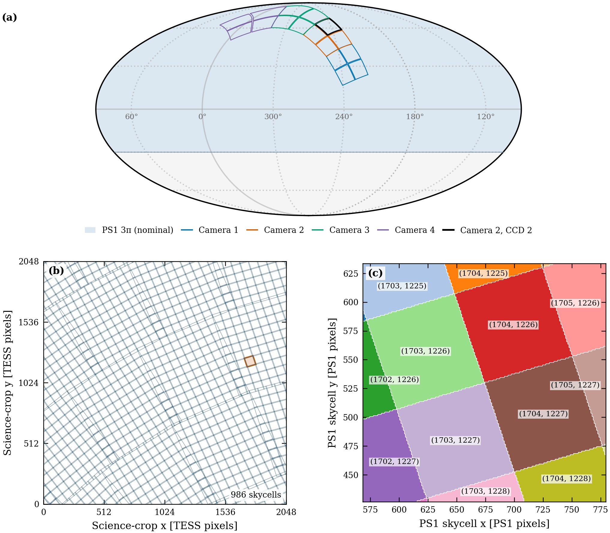
- For every TESS pixel (and sub-pixel) we find the PS1 skycell pixels that cover it, using the initial TESS WCS. Candidate skycells come from a polygon-point query; overlaps are resolved by the nearest PS1 projection centre.
- Each owned TESS pixel's corners are transformed through both WCS solutions, and the enclosed PS1 pixel centres receive its index. The inverse map is stored. A map value of $-1$ means no assignment in that skycell, not necessarily a gap in TESS coverage.
- PS1 values are converted to counts s$^{-1}$ and flux-per-pixel and pixel-area conventions are tracked. The nominal survey footprint is distinguished from valid observed pixels.
(a) Nominal PS1 3π footprint with the Sector 24 camera and CCD outlines; the black outline is camera 2, CCD 2. (b) The 986 skycells that overlap that CCD's 2048×2048-pixel science crop; the coloured (orange) patch marks the skycell shown in (c). (c) A 211×207 PS1-pixel cutout of that skycell (43,677 pixels, all assigned), covering TESS pixels $x=1702$–1705, $y=1225$–1228 of (b). Each coloured region is the set of PS1 pixels assigned to one TESS pixel and is labelled by that TESS pixel’s $(x,y)$ in the frame of (b); the four corner slivers are too small to label. The PS1 pixel scale is 0.25 arcsec and the TESS pixel scale is 21 arcsec.
2.2 Band synthesis
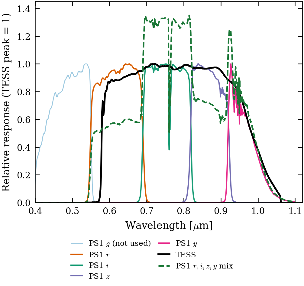
The four PS1 bands are added with fixed weights into one TESS-like image per skycell, $$C_0=\sum_{b\in\{r,i,z,y\}} w_b F_b,\qquad (w_r,w_i,w_z,w_y)=(0.254,\,0.4368,\,0.1654,\,0.1438),$$ where $F_b$ is the PS1 band-$b$ image (counts s$^{-1}$ per pixel) and $w_b$ are dimensionless weights fitted so that the mix reproduces the TESS count rate predicted from Gaia XP spectra. The mix matches TESS only after integration over smooth stellar spectra, not wavelength by wavelength. Residual synthesis errors are listed in Appendix C.
PS1 $r,i,z,y$ response curves (unit peak, including 1.2 airmasses), PS1 $g$ (unused), the TESS response (version 2.0, unit peak) and the weighted mix (dashed), which shares the TESS scale and is scaled so that a G2V star gives the same photon rate through the mix as through the TESS response. The mix is 0.65 of TESS at 600–672 nm, 1.33 at 717–800 nm and 0.65 at 900–910 nm. It is a linear combination of the four PS1 curves, as checked against the stored weights.
2.3 Source removal
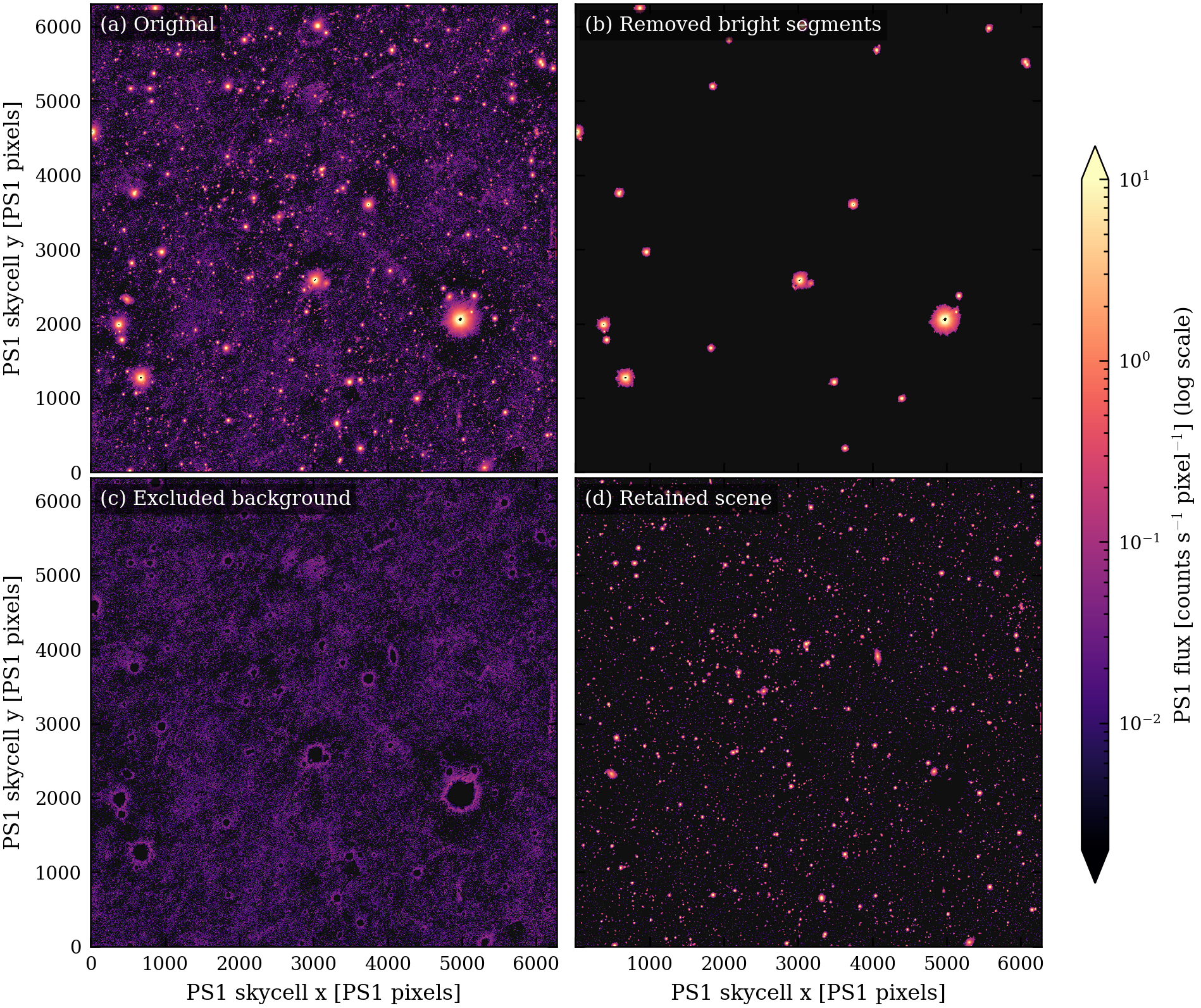
- On the combined image only, we keep the pixels of detected sources and set the PS1 sky to zero, because sky left in would spread under smoothing and rebinning. Invalid chip-gap coverage is treated separately.
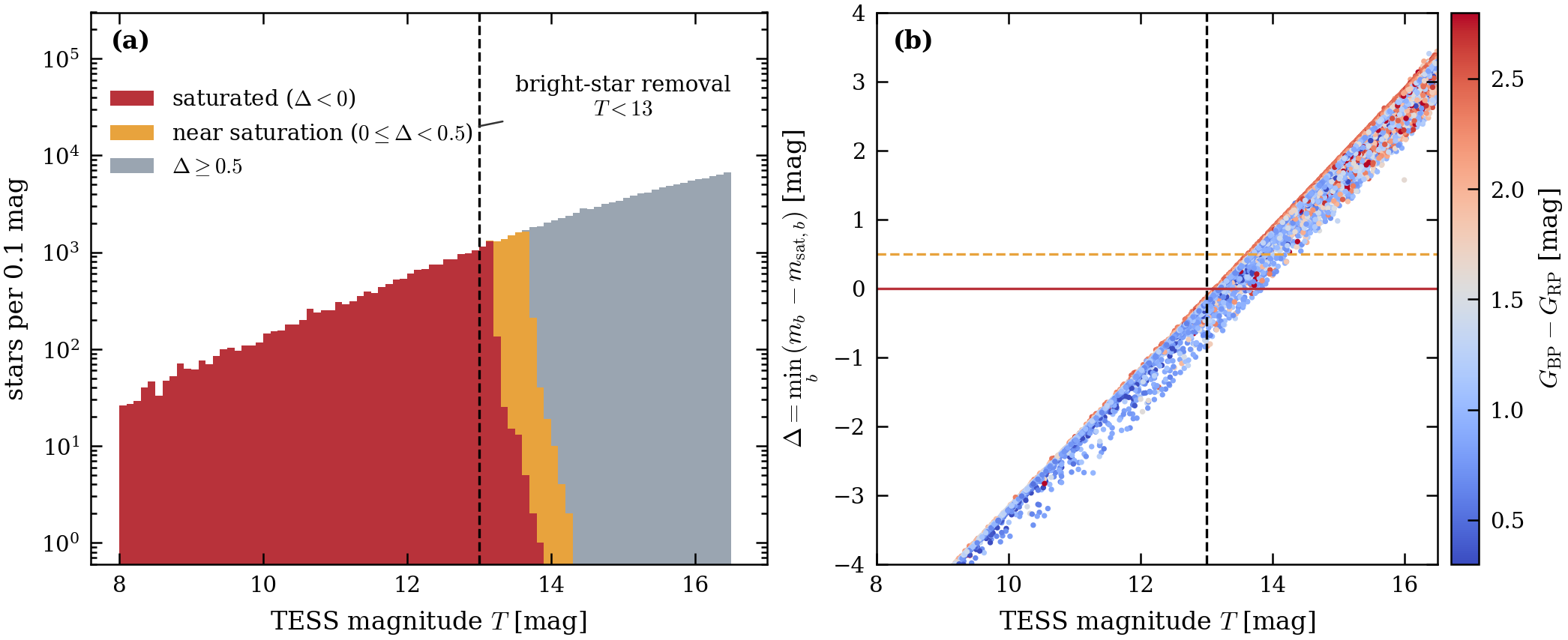
- The whole footprint of every saturated or $T<13$ star is blanked, so that these stars stay in the TESS image and can be fitted.
- On valid pixels, original = removed sources + excluded PS1 background + retained scene.
- Every Gaia star that lies inside a removed (blanked) region is logged together with the region that removed it, including the faint neighbours removed along with a bright star, so the light taken out of the template can be traced star by star.
Skycell 2436.091 (6283×6302 pixels, shown as 8×8 means) with the adopted band weights: (a) the original combination, (b) the bright-source segments removed from the template, (c) pixels excluded as background, (d) the retained scene that becomes the template. The four images sum to the original in every valid pixel, on one logarithmic scale. Against the previous weights the retained flux changes by −1.74 %.
2.4 Smoothing, seams and sampling
- Each weighted band is multiplied by the keep mask and smoothed with one Gaussian ($\sigma=40$ PS1 pixels, 10.3 arcsec), across skycell boundaries with seam corrections, so the single-skycell edge never shows.
- Each smoothed band is binned onto the TESS grid through the mapping, on a grid four times finer than the TESS pixel and at native sampling. The $4\times4$ block sum of the fine grid reproduces the native grid to $10^{-15}$.
- The band templates $T_b$ are summed with their weights already included into $T=\sum_b T_b$.
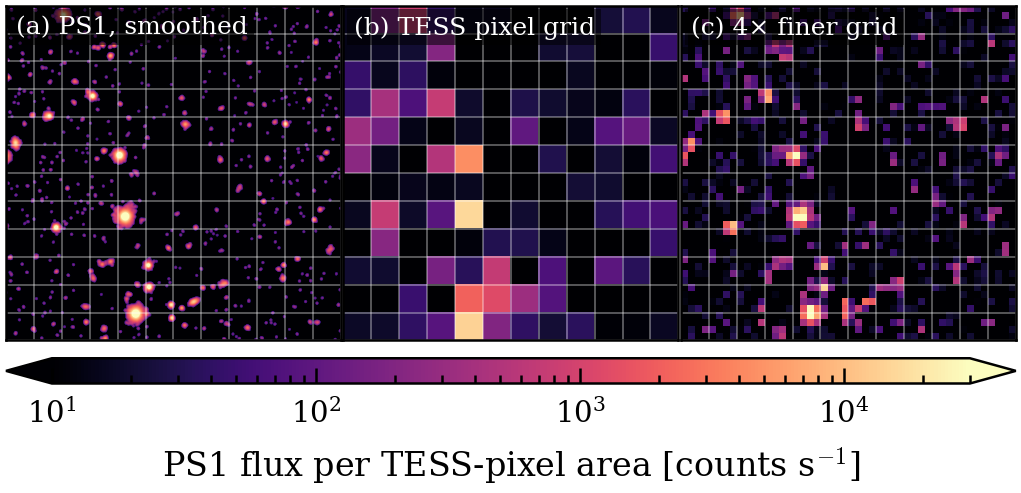
One smoothed PS1 scene (a 1008×1008-pixel cutout, smoothed with $\sigma=2.5$ PS1 pixels for display) at (a) PS1 resolution, (b) integrated onto the TESS pixel grid and (c) integrated onto a grid four times finer. All panels show surface brightness per TESS-pixel area, so cells of different size compare directly; white lines mark TESS pixel boundaries. The block sum of (c) reproduces (b) to a relative $8\times10^{-16}$.
2.5 Photometric calibration of the band templates
The PS1 stack images carry a per-skycell flux-scale error of 0.6–1.7 % per band, coherent over tens of skycells, and the template keeps a small fraction of each star's wing light beyond its segment that catalogue PSF magnitudes do not include. We rescale each band of each skycell by a factor measured on isolated stars. For skycell $s$ and band $b\in\{r,i,z,y\}$, $$\rho_{k,b}=\frac{F^{\rm seg}_{k,b}}{F^{\rm ref}_{k,b}},\qquad M_{s,b}=\operatorname*{med}_{k\in s}\rho_{k,b},$$ where $F^{\rm seg}_{k,b}$ is the flux of star $k$ summed over its own segment in the band template before smoothing (counts s$^{-1}$), and $F^{\rm ref}_{k,b}=10^{-0.4(m_{k,b}-25)}$ is its reference flux from the PS1 DR2 mean PSF magnitude $m_{k,b}$. Stars are isolated Gaia sources with $15\le G\le17.5$ and $0.3\lt G_{\rm BP}-G_{\rm RP}\lt 3.2$, about 50 per skycell. Each $M_{s,b}$ is shrunk toward the median of its neighbouring skycells by the ratio of the intrinsic variance $\tau^2$ (estimated from two independent halves of the star sample) to the total variance, giving $\hat M_{s,b}$; this changes individual skycells by less than 0.3 %.
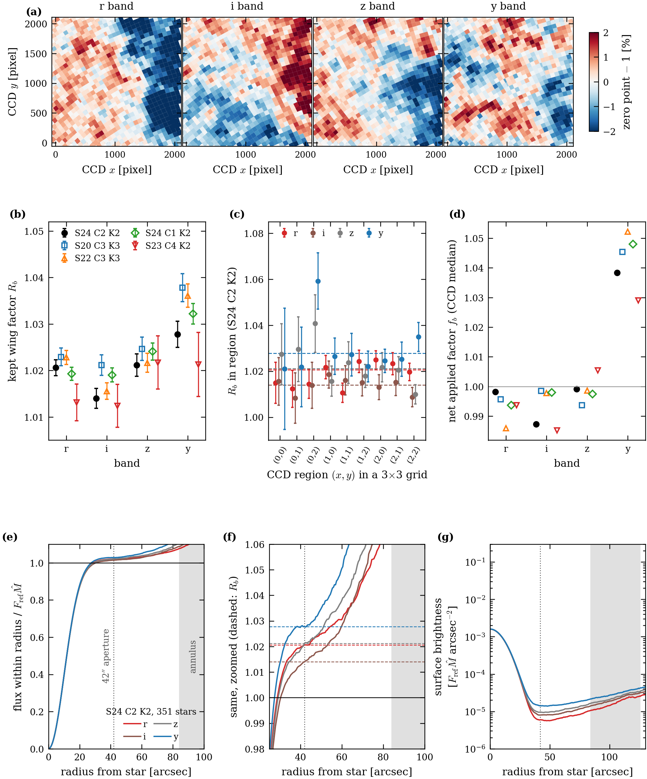
The kept wing fraction is one number per band and CCD, $$R_b=\operatorname*{med}_{k}\frac{S_{k,b}}{F^{\rm ref}_{k,b}\,\hat M_{s(k),b}},$$ where $S_{k,b}$ is the star's flux within 42 arcsec in the smoothed band template minus the local annulus level (84–126 arcsec), measured on template stars with $13.6\le T<15.5$. Here the reference flux is the Gaia $(G,\,G_{\rm BP}-G_{\rm RP})\rightarrow$ PS1 transform, which has twice as many template stars as the PS1 catalogue: the per-skycell structure comes from PS1 and the per-band level from Gaia. We find $R_b=1.012$–$1.025$ for $r,i,z$ and $1.021$–$1.038$ for $y$, uniform across each CCD within noise.
Each band template is rebuilt as $T'_b=\sum_s C_{s,b}/f_{s,b}$ with $f_{s,b}=\hat M_{s,b}R_b/g$, where $C_{s,b}$ is skycell $s$'s contribution to band $b$ and $g$ is the median of $\hat M R$ over skycells and bands, so the overall scale of each field is unchanged. The net per-CCD effect is a factor $1.029$–$1.052$ in $y$ and $0.985$–$1.005$ in $r,i,z$. The calibration brings the template band ratios to within 0.5 % of the Gaia-XP colours and removes the $y$ excess at every colour. It is applied to the band templates before they are combined, so it enters both the preliminary template and the final per-band templates. The calibration changes the total template flux of red relative to blue stars by only −0.6 %, so it does not explain the red total-flux deficit of §6. It acts together with the kernel shift for the PS1 stack offset (§5.2): the shift corrects the stacks' astrometric offset and the calibration the per-band zero-point error. With the shift alone the achromatic dipole of mid-colour stars is 4.9–8.4 mpx; with both it is 0.8–5.5 mpx (Fig. 21).
Numbers marked here come from the hybrid factors and are to be refreshed from the final production run.
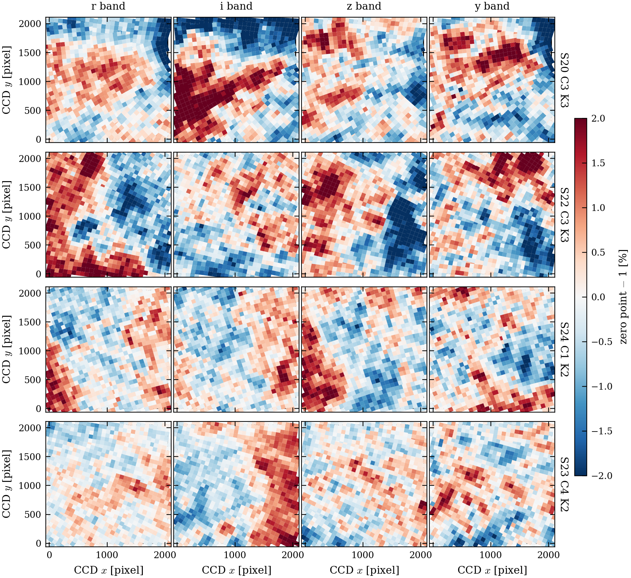
(a) Per-skycell zero point of the $r,i,z,y$ templates for S24 camera 2 CCD 2, relative to its CCD median, coherent over tens of skycells with an rms of 0.9–1.2 % per band. (b) Kept wing factor $R_b$ for five CCDs: 1.013–1.025 in $r,i,z$ and 1.021–1.038 in $y$, with 0.14–0.7 % uncertainties. (c) $R_b$ in nine CCD regions of S24 C2 K2; regions agree with one value per CCD (reduced $\chi^2$ 0.3–1.2), the largest deviation (about 2$\sigma$) is common to all bands. (d) Net factor $f_{s,b}$ per band as the CCD median: 0.986–1.005 in $r,i,z$ and 1.029–1.052 in $y$. (e) Median curve of growth of the 351 stars behind $R_b$ in S24 C2 K2 ($13.6\le T<15.5$, least crowded 30 %), in each smoothed band template, divided by the catalogue flux $F^{\rm ref}\hat M$, with the median annulus level (84–126 arcsec, grey) subtracted; dotted: the 42-arcsec aperture. (f) The same, zoomed: the value at 42 arcsec is the kept wing factor $R_b$ (dashed), 1.4–2.8 % above the catalogue flux. (g) Median surface brightness of the smoothed template around the same stars. The curve has no flat plateau: beyond about 45 arcsec it keeps rising, because the surface brightness climbs toward the annulus with the light of neighbouring stars, which the median annulus level does not remove. $R_b$ is therefore defined at the 42-arcsec aperture, and a wider aperture would give a larger value.
Supplement: per-skycell maps for all fields
The five fields and the recipe used throughout. The calibration of §2.5 is applied to the band templates before they are combined, for both the preliminary and the final template.
Part 1: data
| Image | FFI file | UTC start | Exposure start (TSTART, BTJD) | Camera/CCD | Crop origin (x,y), size | PS1 skycells | Stars fitted (T≤13) | Held-out cores | Colour $u-u_{\rm ref}$ 5-95% | Median image-level background (e-/s) |
|---|---|---|---|---|---|---|---|---|---|---|
| F1: S24 C2 K2 | tess2020120182919-s0024-2-2-0180-s_ffic.fits.fz | 2020-04-29T18:30:52.206 | 1969.2722 | 2/2 | (44,0), 2048x2048 | 986 | 14,733 | 10,536 | -0.31 … +0.49 | 65.6 |
| F2: S20 C3 K3 | tess2020013215923-s0020-3-3-0165-s_ffic.fits.fz | 2020-01-13T22:01:56.377 | 1862.4188 | 3/3 | (44,0), 2048x2048 | 999 | 15,521 | 8,767 | -0.31 … +0.51 | 70.9 |
| S22 C3 K3 | tess2020071012921-s0022-3-3-0174-s_ffic.fits.fz | 2020-03-11T01:31:54.518 | 1919.5646 | 3/3 | (44,0), 2048x2048 | 976 | 12,543 | 8,491 | -0.30 … +0.49 | 72.7 |
| C1: S24 C1 K2 | tess2020118235919-s0024-1-2-0180-s_ffic.fits.fz | 2020-04-28T00:04:03.780 | 1967.5036 | 1/2 | (44,0), 2048x2048 | 944 | 10,984 | 8,224 | -0.31 … +0.53 | 84.5 |
| C4: S23 C4 K2 | tess2020087042920-s0023-4-2-0177-s_ffic.fits.fz | 2020-03-27T04:30:06.872 | 1935.6884 | 4/2 | (44,0), 2048x2048 | 975 | 19,120 | 13,528 | -0.32 … +0.47 | 80.8 |
Part 2: recipe
| Setting | Value |
|---|---|
| Background-estimate template | Template on the TESS-pixel grid (native sampling) |
| Preliminary and final images: template | Template on a grid 4 times finer than TESS pixels |
| Band weights (r,i,z,y) | 0.254, 0.4368, 0.1654, 0.1438 |
| PS1 Gaussian pre-smoothing sigma | 40 PS1 pixels (10.3 arcsec) |
| Bright-star removal limit | T<13 (removed from the PS1 template) |
| PS1 calibration | per-skycell zero point x per-CCD kept-wing factor, applied to the final per-band templates only |
| Background method | Magnitude-sized wing exclusion (30 px at T<6.15 down to 6 px at T<13); harmonic gap fill |
| Preliminary image (Hotpants) | kernel spatial order 4; no background term (background order -1); 3 Gaussians, sigma = 0.752, 1.88, 3.76 px |
| ePSF grid | 6x6 nodes, 4x oversampled, pixel-integrated |
| WCS model | Tangent plane + degree-5 Chebyshev (21 terms per axis, 42 coefficients) |
| Colour model | Radial shift (knots 0, 0.7, 1.5, 3.0, 5.5 px) and coma (knots 0.4, 0.8, 2.2, 5.0 px) basis, tapered to zero at 7 px; 53 coefficients |
| Regularisation | Local-polynomial prior weight $3\times10^{8}$, window 7x7 pixels (orders 4,2,1; radii 3,5); Laplacian weights 0.01 |
| Brightness-width term | None |
| Folds | K=5 spatial folds (128-px tiles, diagonal pattern) |
| Stopping rule | A stage ends when the 50-step mean loss has fallen by less than $10^{-4}$ (relative) over the last 500 steps, the largest star-position change over those steps is below 0.5 mpx and the median relative flux change is below $10^{-4}$ (checked every 100 steps, after at least two learning-rate decays); at most 3000, 20000 and 20000 steps in the three stages |
Note: time is TSTART; the PS1 calibration is applied to the final per-band templates only, and the fit on the preliminary image (Secs. 4-5, Table 3) is uncalibrated by design.
3 Preliminary de-crowded image
3.1 Template match
Hotpants matches the band-combined template to the science frame with a spatially varying kernel, and the matched template is subtracted: $$D_{\rm prel}=(I-B)-K\ast T,\qquad T=\sum_b T_b .$$
- $D_{\rm prel}$: preliminary de-crowded image (native pixels, e$^-$ s$^{-1}$).
- $I$: the FFI (e$^-$ s$^{-1}$); $B$: the image-level background of §3.2.
- $T$: band-combined template on the grid four times finer than the TESS pixel, integrated onto native pixels, with the band weights included (§2.4). It is built from the calibrated band templates (§2.5).
- $K$: the fitted kernel, which also sets the flux scale. Basis of three Gaussians ($\sigma=0.752,\,1.88,\,3.76$ px) each times a polynomial; spatial order 4; no polynomial background term; stamps built from connected unmasked regions.
Stars brighter than $T=13$ were removed from the template and so remain in $D_{\rm prel}$; they are the stars we fit in §4.
3.2 Image-level background
The science frame carries a smooth additive background (scattered light, sky) and the wings of bright stars. We alternate between fitting a kernel and estimating an image-level background $B(x,y)$ on the star-subtracted residual, and subtract $B$ before the final Hotpants run.
- Kernel fit, round 1. Hotpants matches the template $T$ to the science frame $I$ with a kernel $K$ and a third-order polynomial background $b_0(x,y)$: $$I \simeq K\otimes T + b_0 .$$ Only $K\otimes T$ is kept; $K$ is fitted and $b_0$ is discarded. The frame used is the sector's lowest-background exposure.
- Residual and fit pixels. The residual is $D_1=I-K\otimes T$ (e$^-$ s$^{-1}$). Background-fit pixels are those with no mask flag other than the faint-star flag (strap columns, bright-star crosses and saturation, catalogue-star circles, transients and asteroids are excluded), minus magnitude-sized disks centred on every catalogue star with $T_{\rm mag}<13$. The disk radius falls from 30 native pixels at $T_{\rm mag}<6.15$ to 6 pixels at $T_{\rm mag}<13$: it is the radius at which the fitted azimuthal wing of the star falls below $\tau=0.1$ e$^-$ s$^{-1}$ ($\tau$ is a fixed constant). The disks affect only the background fit, never the Hotpants fit.
- Background on the residual. Fit pixels that border a masked region and deviate from their 15 nearest valid neighbours by more than $3\sigma$ (robust MAD) are also dropped. Masked pixels are filled by solving Laplace's equation, $$\nabla^2 B_{\rm fill}=0 \ \ \text{in masked regions},\qquad B_{\rm fill}=D \ \ \text{on the fit pixels},$$ where $D$ is the residual and $B_{\rm fill}$ the filled map (e$^-$ s$^{-1}$). The maximum principle bounds the fill by its rim values, so it cannot overshoot. The map is smoothed with a Gaussian ($\sigma=2$ px, widened by a factor 4 on low, flat residuals), isolated anomalies are repaired against a 16-pixel-box median background, and a per-column quantum-efficiency spline is applied in strap columns. The result is $B_1$.
- Alternate. The kernel is refitted on $I-B_1$ with the Hotpants background switched off, giving $D_2=I-K_2\otimes T$ and $B_2$ by the same estimator. A third kernel fit on $I-B_2$ (background off) gives the final kernel $K$: three kernel fits and two background estimates in all.
- Science-frame background. $K$ is applied to the template and the same estimator gives $$B=\mathcal{E}\left[I-K\otimes T\right],$$ where $\mathcal{E}$ is the estimator of step 3.
- Final Hotpants. Hotpants matches the finer-grid template to $I-B$, integrating it onto native pixels, with kernel spatial order 4, no polynomial background, and stamps from connected unmasked regions. The output is $D_{\rm prel}$ of §3.1.
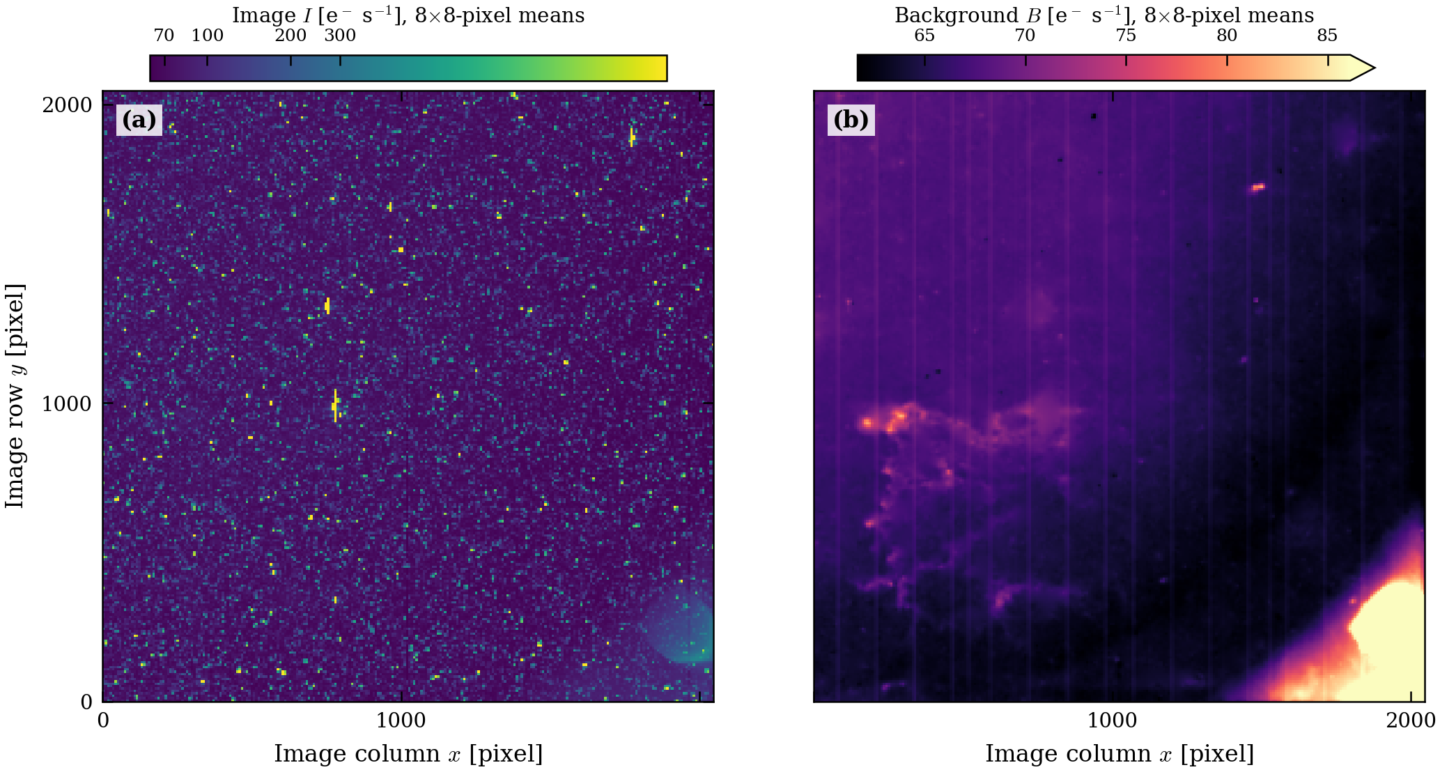
(a) Image $I$ over the full CCD (2048×2048 pixels, 8×8 area means, logarithmic). (b) Background $B$ on the same grid (61.7 to about 85 e$^-$ s$^{-1}$; scattered light raises the lower-right corner to 372 e$^-$ s$^{-1}$ in 8×8 means).
3.3 Before and after
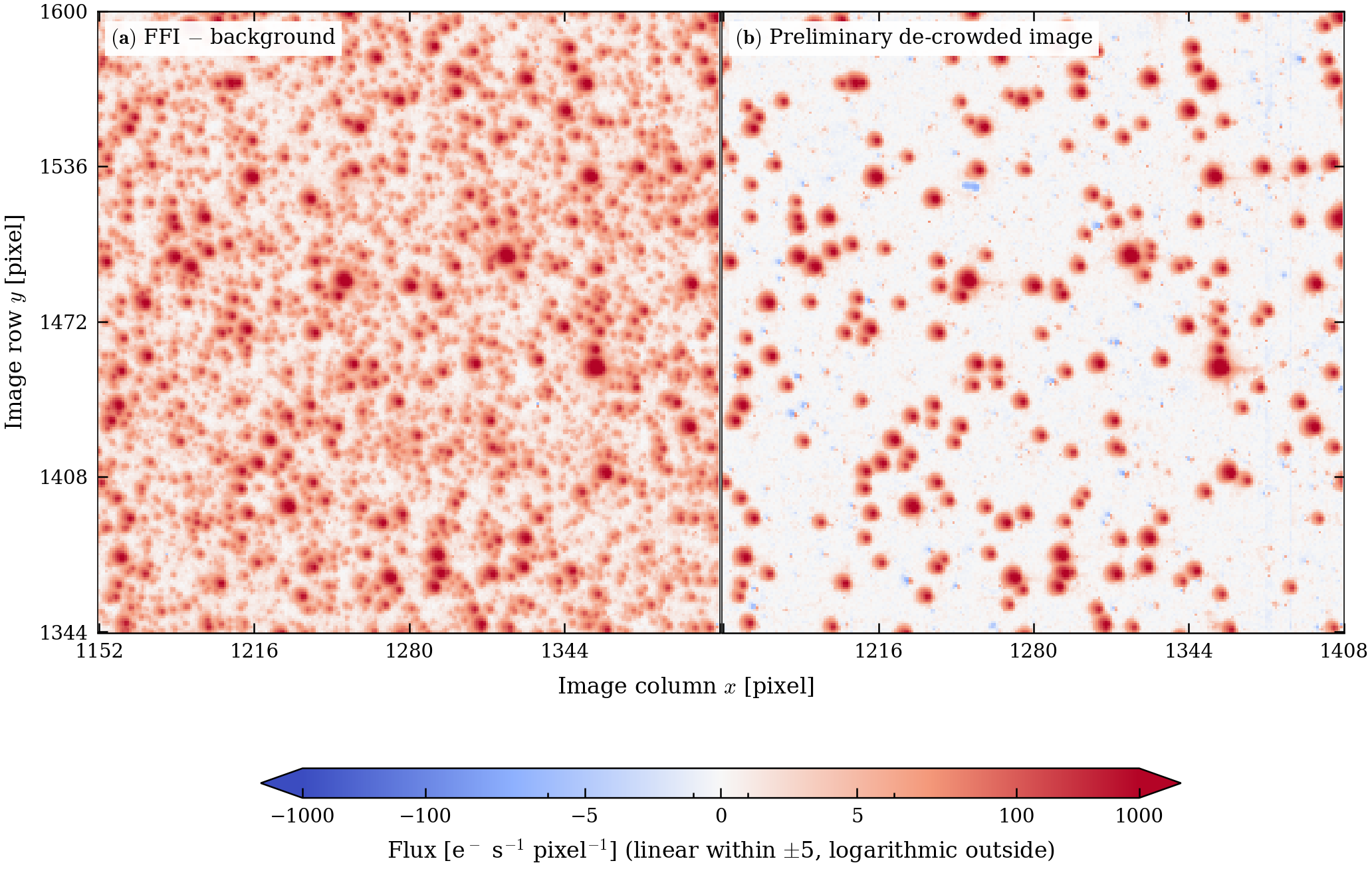
- The background-subtracted FFI and its preliminary de-crowded image are shown at identical coordinates and display limits.
- Reduced crowding motivates the scene fit. A cleaner picture alone does not establish unbiased flux or astrometry; those are tested in §4 and §5.
Single-frame crop (256×256 pixels) of the S24 camera 2 CCD 2 frame. (a) The full-frame image minus the background $B$. (b) The preliminary de-crowded image, on the same colour scale: linear within $\pm5$ e$^-$ s$^{-1}$ per pixel, logarithmic outside, clipped at $\pm10^3$. Stars fainter than $T\approx13$ are in the template and are subtracted, leaving only noise; brighter stars are removed from the template (§2.3) and remain unchanged.
4 Joint fit and the TESS ePSF
All bright Gaia stars in $D_{\rm prel}$ are fitted together for the WCS, a spatially and colour-dependent ePSF, and fluxes. There is no fitted background.
One joint fit gives the WCS, a spatially and colour-dependent ePSF and the fluxes. Each subsection gives how a dependence is modelled and then what is measured on held-out stars; the brightness dependence is measured but not modelled (§4.6).
4.1 Scene model and likelihood
$$m_p=\sum_i f_i\,R_{ip},\qquad \mathcal L=\sum_{p}\frac{(D_p-m_p)^2}{\sigma_p^2},\qquad \boldsymbol x_i=W\!\left(\boldsymbol s_i(t_{\rm exp});\boldsymbol a\right)+\Delta\boldsymbol x_i(\delta_i,\boldsymbol r_i)$$
- $m_p$: model value of native pixel $p$ (e$^-$ s$^{-1}$); $D_p$ the data in the preliminary image; $\sigma_p$ the pixel noise from the image's noise plane; $\mathcal L$ the weighted squared residual summed over unmasked pixels; the ePSF smoothness prior of §4.5 is added to it.
- $f_i$: flux of star $i$ (e$^-$ s$^{-1}$), solved by linear least squares at fixed shared parameters.
- $R_{ip}$: response of pixel $p$ to star $i$ (§4.4), zero outside the star's finite support.
- $\boldsymbol x_i$: crop-local pixel position; $\boldsymbol s_i(t_{\rm exp})$: Gaia DR3 position propagated to the exposure epoch.
- $W$: reference-colour WCS (§4.2) with fitted coefficients $\boldsymbol a$.
- $\Delta\boldsymbol x_i$: colour-dependent displacement (§4.5), a function of the colour offset $\delta_i$ and detector position $\boldsymbol r_i$.
Stars to $T\le13$ are fitted. Straps are masked, and there is no data-dependent rejection inside the fit.
Fainter neighbours are carried in the model as nuisance sources. Gaia stars with $13 These are mainly faint stars blanked from the template together with a bright neighbour, whose light therefore remains in $D_{\rm prel}$. Stars fainter than $T=17$ are not modelled.
4.2 WCS and centroid gauge
- The WCS is a tangent plane plus a degree-5 Chebyshev correction (21 terms per axis, 42 coefficients), fitted to Gaia positions propagated to the observation epoch.
- A WCS shift and a shift of the ePSF core centroid are degenerate. The ePSF core centroid is therefore constrained (a gauge condition), and what we report as star-position accuracy is the effective position, the WCS position plus the ePSF centroid.
- The WCS field itself is not an accuracy measurement. Accuracy is measured on held-out stars against Gaia (§5.4).
4.3 Held-out evaluation
- Every accuracy we quote is held out: $K=5$ spatial folds (128-pixel tiles in a diagonal pattern); each star is scored with the fit of the four folds that did not contain it. Delivered calibrations use all stars.
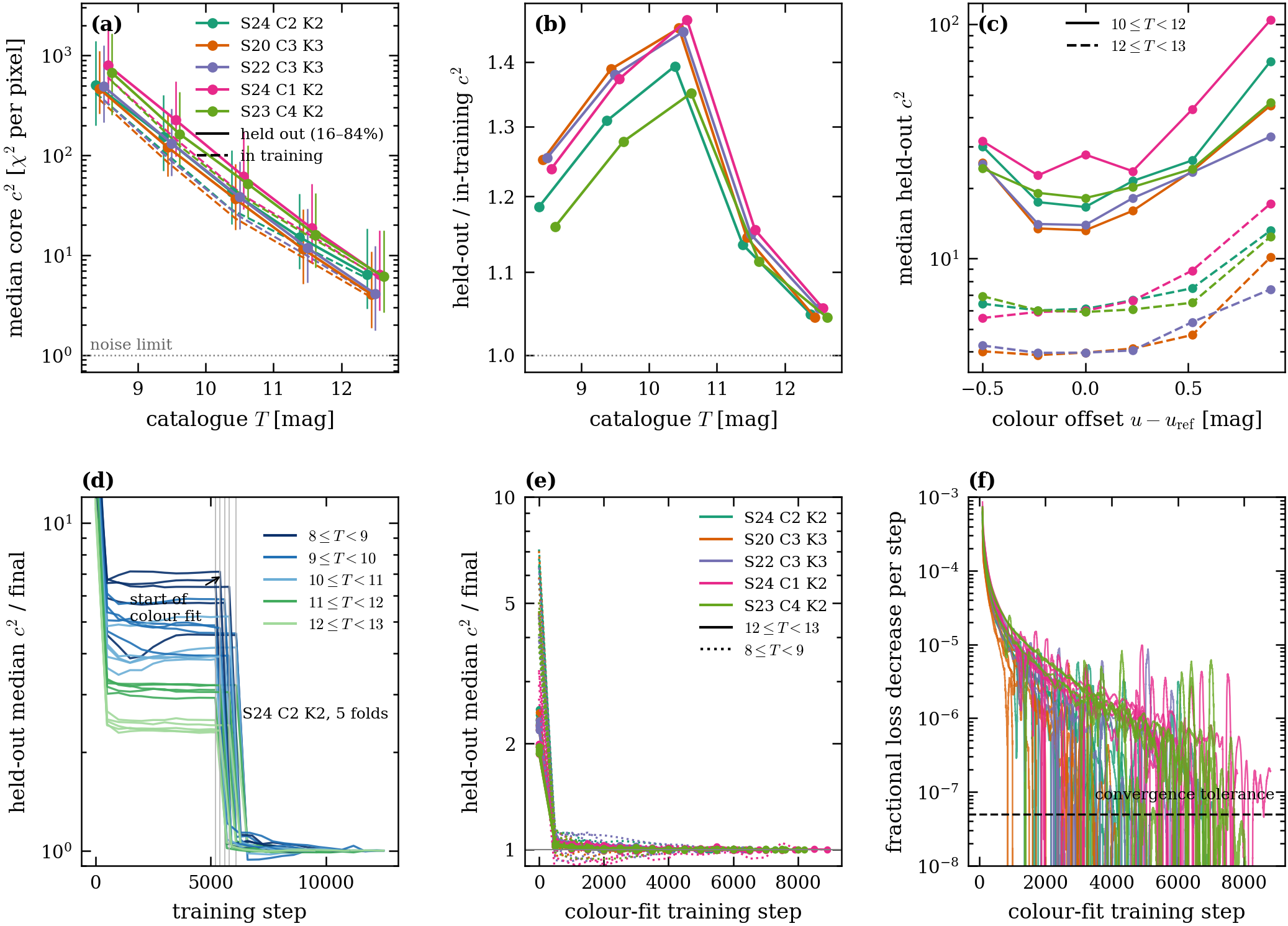
- Stopping rule: a stage ends when the 50-step mean loss has fallen by less than $10^{-4}$ (relative) over the last 500 steps, the largest star-position change over those steps is below 0.5 mpx and the median relative flux change is below $10^{-4}$ (checked every 100 steps, after at least two learning-rate decays), or at the step cap (3000, 20000 and 20000 steps in the three stages).
- Baselines are external: the FFI header WCS and Gaia-XP synthetic photometry.
4.4 Spatial dependence
The ePSF is stored on a $6\times6$ grid of nodes across the CCD, sampled at $O=4$ samples per native pixel and already integrated over pixel area. A star's ePSF is the bilinear blend of the four nearest nodes with the colour terms of §4.5 applied. The pixel value is $$\boldsymbol g_{ip}=\boldsymbol c_E+O\,(\boldsymbol x_p-\boldsymbol x_i),\qquad R_{ip}=O^2\,\mathcal{B}\!\left(E_i,\boldsymbol g_{ip}\right).$$
- $\boldsymbol g_{ip}$: position, in ePSF grid samples, at which star $i$'s ePSF is read for pixel $p$; $\boldsymbol c_E$: grid index of the ePSF centre.
- $\boldsymbol x_p$: centre of native pixel $p$; $\boldsymbol x_i$: star position (§4.1), in crop-local pixels.
- $E_i$: the pixel-integrated ePSF at star $i$'s position and colour; $\mathcal B$: bilinear interpolation from the four nearest samples, zero outside the support.
Stellar centres stay continuous: they are never rounded to quarter-pixel phases. There is no second sub-pixel sum, because $E$ already includes pixel integration. The ePSF grid factor $O$ is independent of the template sampling.
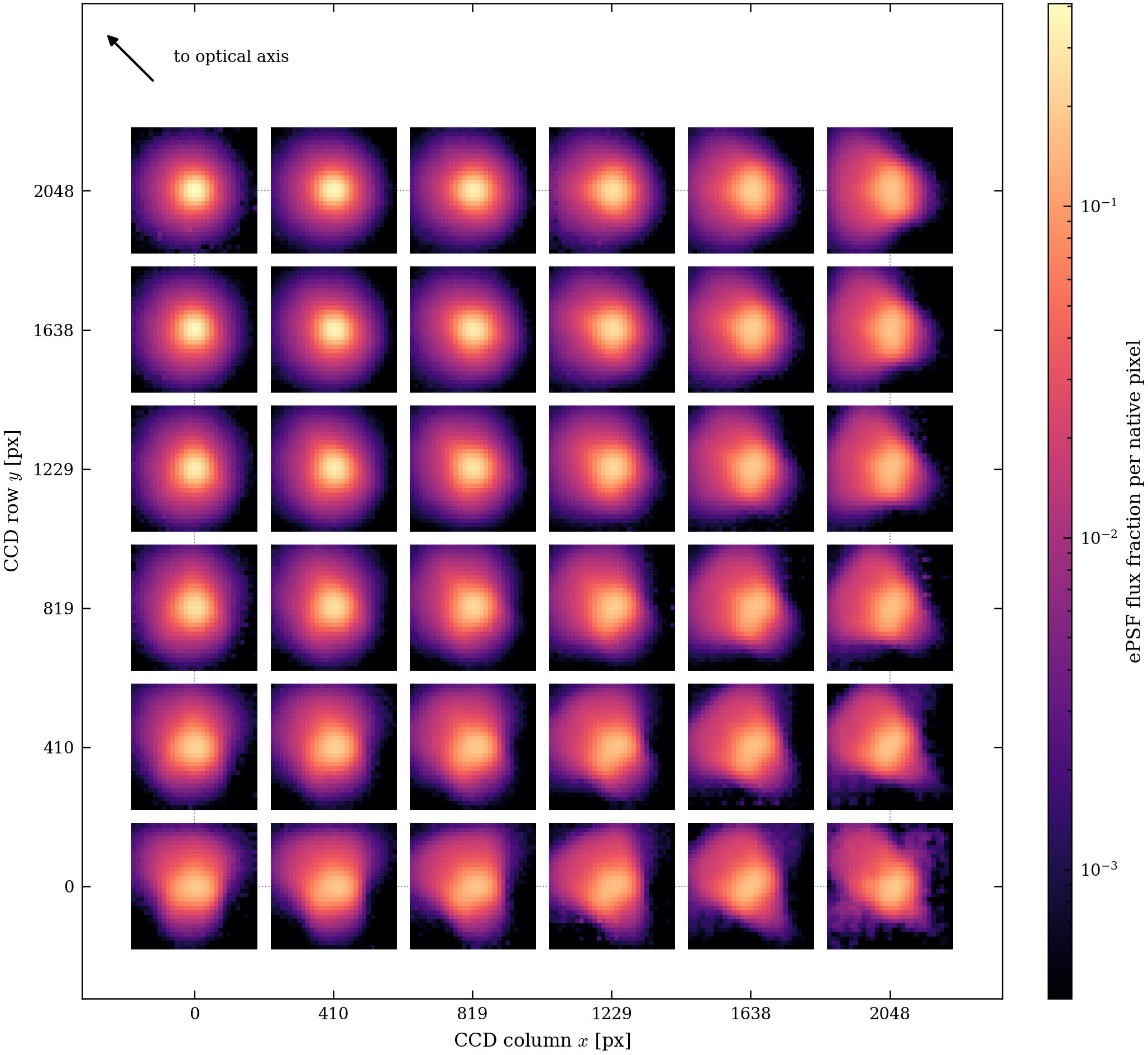
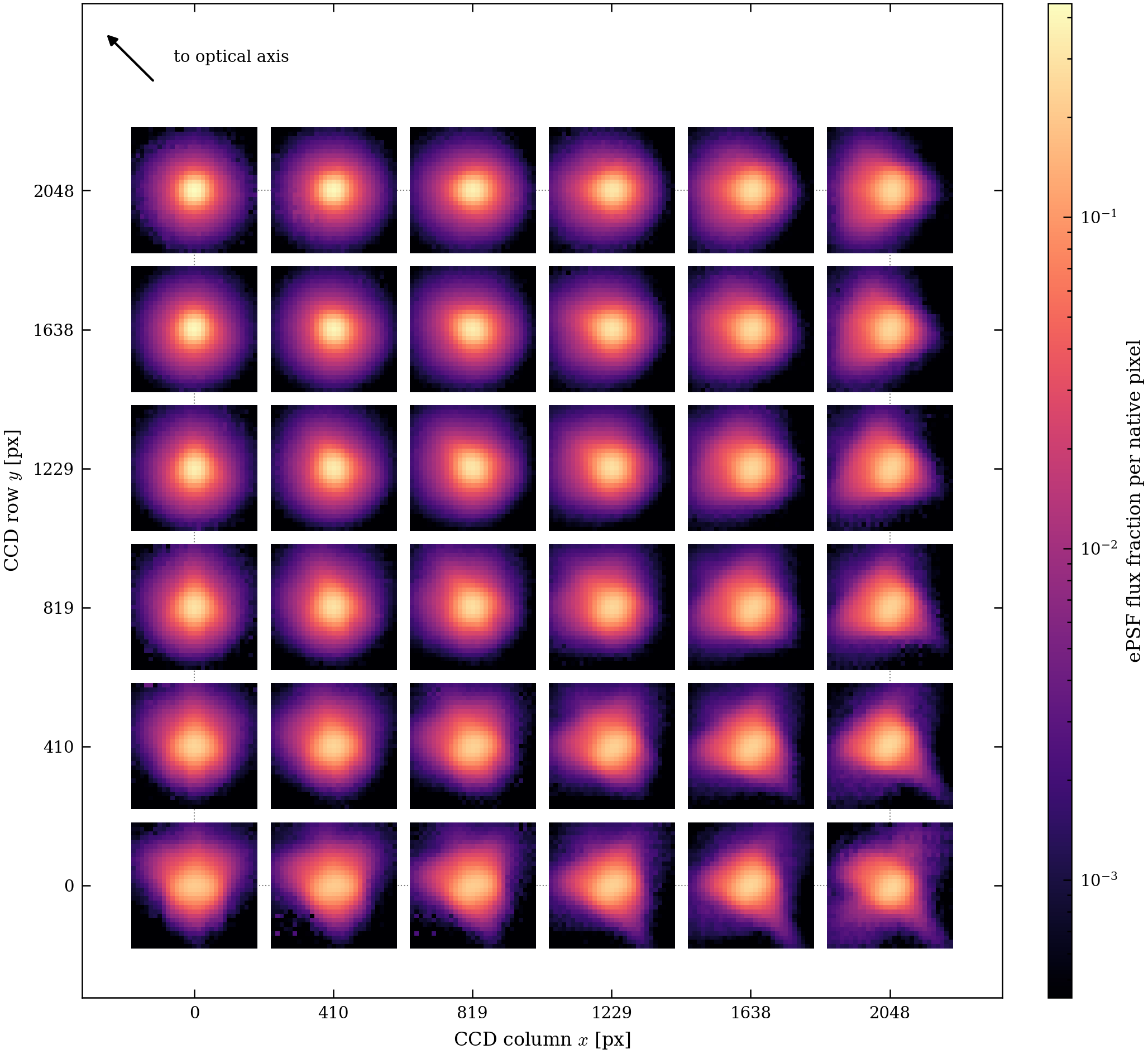
- The spatial change of the ePSF across the detector is 8.8–15.2 times the fold-to-fold scatter across the five fields (median over nodes of the node rms deviation divided by the fold scatter). The fold scatter is the noise of the measurement, so the spatial change is real.
- The rms width is 0.76–1.00 px with ellipticity up to about 0.17, rising toward the far corner of the CCD.
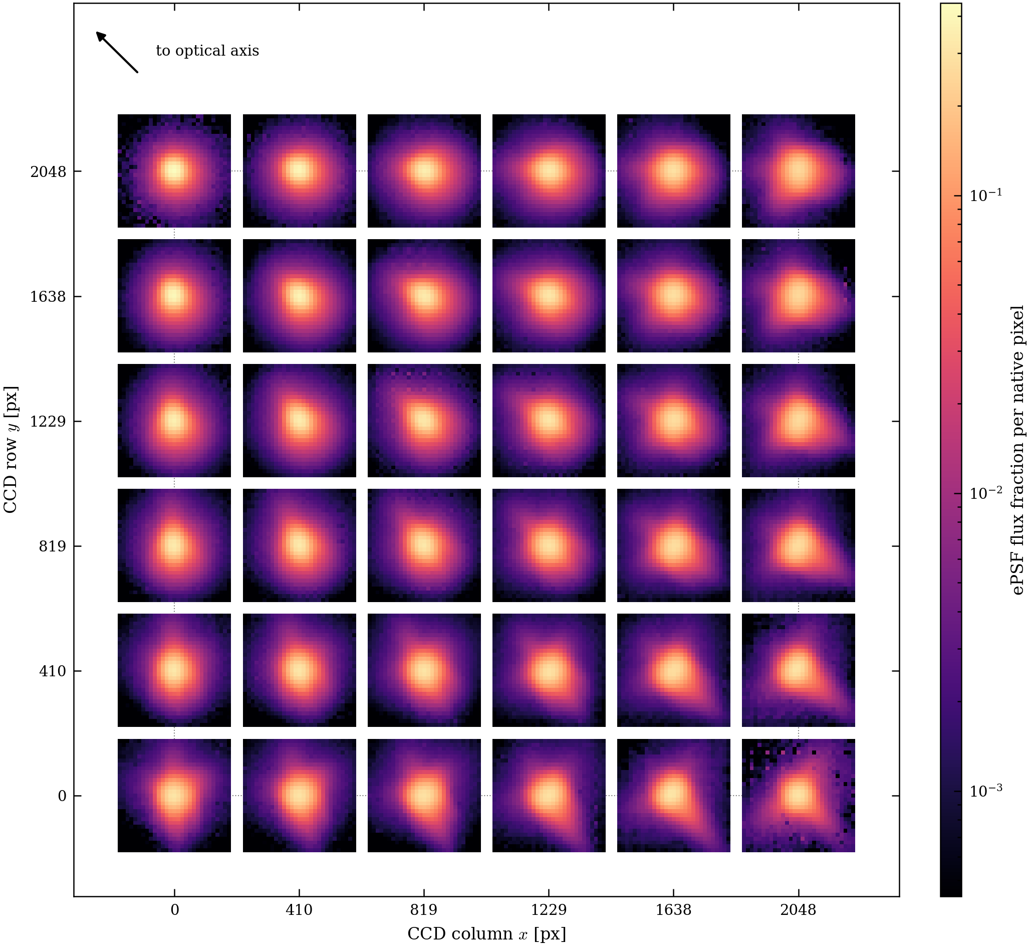
- The same CCD observed in two sectors (F2, S22) largely repeats the pattern: the F2 minus S22 difference has an rms of $2.2\times10^{-3}$ per native pixel, against $8.2\times10^{-3}$ for the node pattern and $0.8$–$1.1\times10^{-3}$ for the fold scatter.
The fitted ePSF of S24 C2 K2 at each node of the $6\times6$ grid, placed at its position on the CCD, from the joint fit to the preliminary image at the reference colour. Each tile spans ±3.5 native pixels at four samples per pixel; all tiles share one logarithmic colour scale over three decades below the brightest node peak. The arrow points to the optical axis: the ePSF is most compact and round nearest the axis and becomes broader and asymmetric toward the far corners.
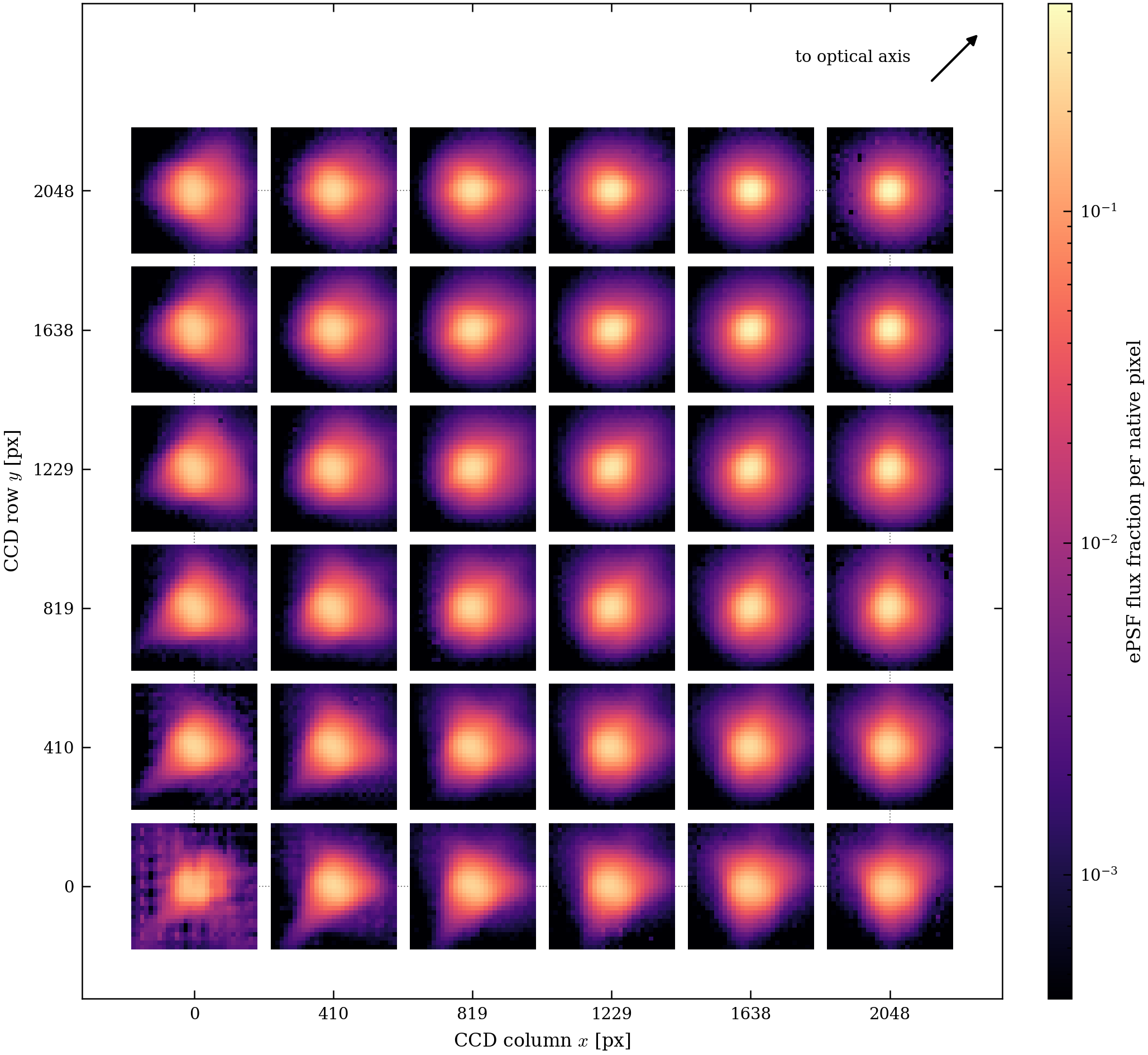
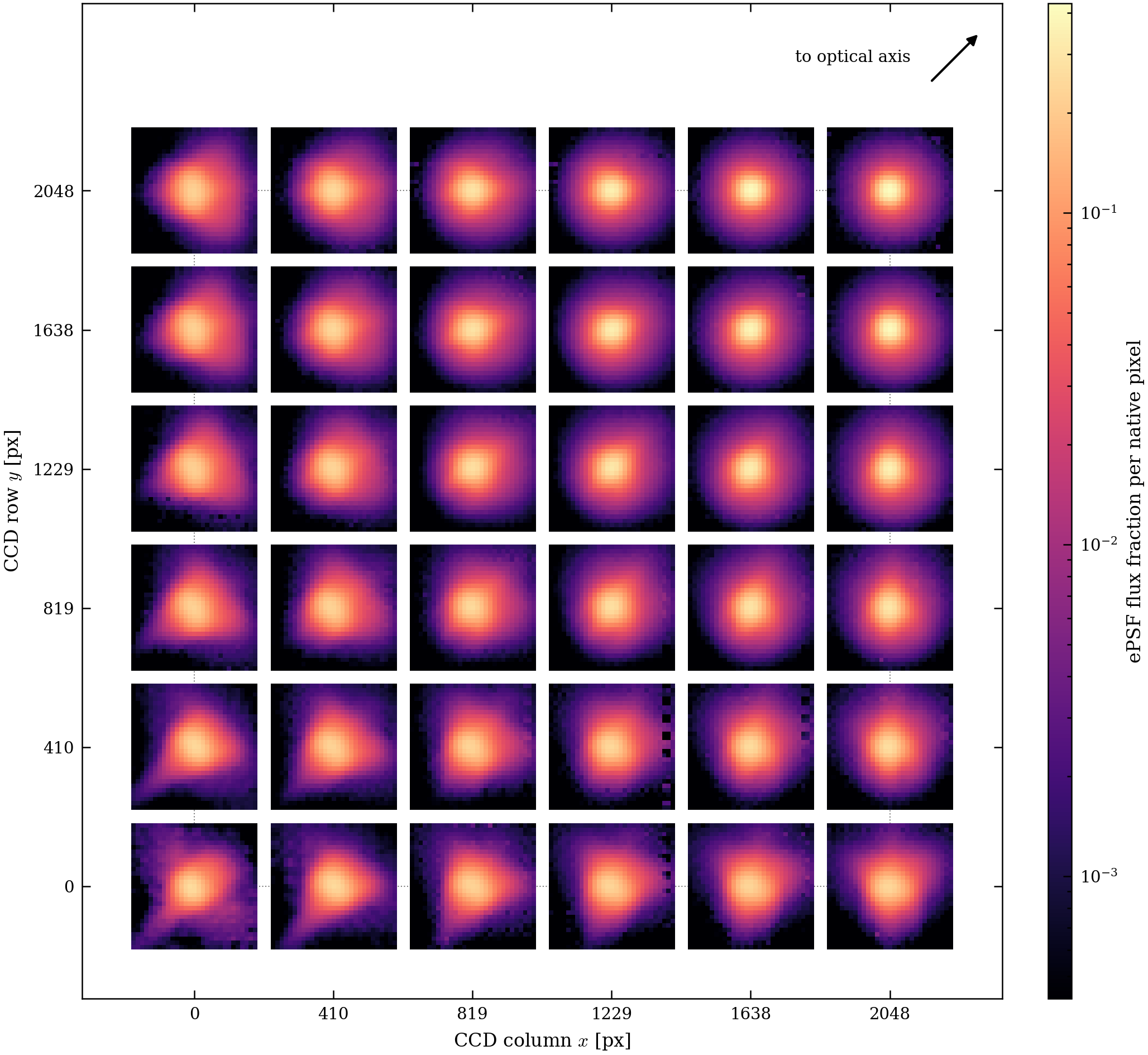
Other fields (S20 C3 K3, S22 C3 K3, S24 C1 K2, S23 C4 K2)
4.5 Colour dependence
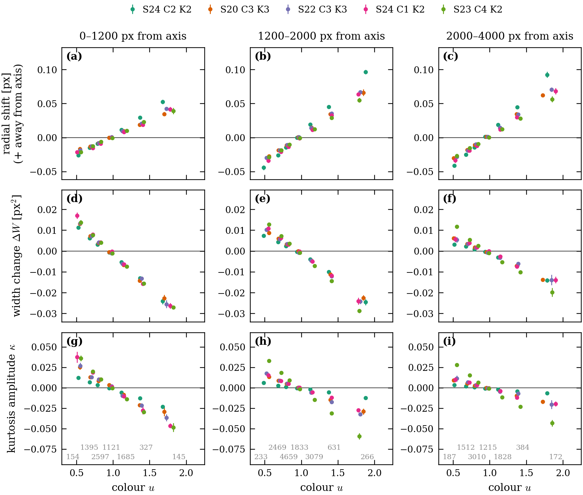
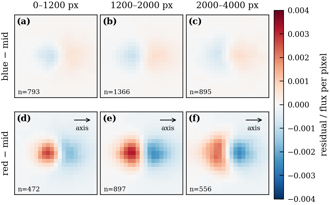
- What the data show, without a model. We fit each held-out star's own response freely. Red stars lie farther from the optical axis, by an amount that grows with axis distance; they have a narrower, peakier core; and a coma-like asymmetry changes sign with radius (Fig. 9). The red minus blue radial shift is $-41$ to $-66$ mpx across the five fields (Table 4).
(a–i) Radial shift, width change $\Delta W$ and kurtosis amplitude $\kappa$ of clean held-out $T=10$–13 stars against colour $u$, in three zones of distance from the optical axis, for five fields. Points: median per colour bin with resampling errors. Each star's value is its own fitted response (the model's colour term plus a free per-star correction), and the slopes agree to 0.2 % (shift) and 1–4 % (width, kurtosis) between the two colour models, so the trends are a property of the data. (j) Stacked (data minus achromatic ePSF)/flux, red minus mid-colour and blue minus mid-colour, five fields pooled, per zone, with the optical axis to the right.
Images behind the curves: stacked residuals by colour
The model that describes these dependences is defined next.
The colour offset is $\delta=u-u_{\rm ref}$, where $u$ is the Gaia XP band-mix colour on the Gaia $G_{\rm BP}-G_{\rm RP}$ scale (the catalogue colour where no XP spectrum exists) and $u_{\rm ref}$ one global reference, defined by $$F_b=10^{-0.4\,m_b},\quad s_b=\frac{v_bF_b}{\sum_{b'}v_{b'}F_{b'}},\quad \Lambda=\sum_b s_b\lambda_b,\quad u=\alpha+\beta\Lambda,\quad u_{\rm ref}=\langle u\rangle_{\rm fit},$$ where $u$ falls back to the catalogue $G_{\rm BP}-G_{\rm RP}$ for a star with no XP spectrum. The colour-dependent change of the ePSF is a radial shift plus a sum of basis functions: $$P_i(\boldsymbol\xi)=P_0\!\left(\boldsymbol\xi-\Delta\boldsymbol x_i\right)+\Delta P_i(\boldsymbol\xi),\qquad \Delta P=\sum_{j=1}^{5} a_j\,G^{\rm rad}_j+\sum_{k=1}^{4} c_k\left(n_x\,G^{\rm com}_{k,x}+n_y\,G^{\rm com}_{k,y}\right),$$ $$\Delta\boldsymbol x=\delta\,s(r)\,\hat{\boldsymbol n}.$$
- $m_b$: synthetic Pan-STARRS1 magnitude of the star in band $b\in\{r,i,z,y\}$, computed from its Gaia XP spectrum (standardised PS1 system); $F_b$ the corresponding flux; $v_b=(0.238,0.344,0.283,0.135)$ fixed weights that define the colour (an earlier band mix, kept so the colour scale does not change; they are not the template weights $w_b$ of §2.2); $s_b$ the share of the star's weighted light in band $b$.
- $\Lambda$: the band-mix wavelength (nm), the share-weighted mean of the band wavelengths $\lambda_b=(617,752,866,962)$ nm.
- $\alpha$, $\beta$: a straight-line fit of Gaia $G_{\rm BP}-G_{\rm RP}$ against $\Lambda$ over the stars of the scene that have both, done once per scene; it puts $\Lambda$ on the $G_{\rm BP}-G_{\rm RP}$ scale ($\beta=0.0343$–0.0350 mag per nm in the five fields).
- $u_{\rm ref}$: the unweighted mean of $u$ over the fitted stars (ePSF-contributor and anchor roles, $T\le13$); one number for the whole scene.
- $P_0$: the ePSF at the reference colour (§4.4); $\boldsymbol\xi$: coordinate on the ePSF grid (not the colour $u$).
- $\Delta\boldsymbol x$: lateral colour shift of the star's light, along $\hat{\boldsymbol n}=(n_x,n_y)$, the unit vector from the star toward the optical axis; $r$ is the distance to the optical axis (px) and $s(r)$ a fitted smooth function of it (px per unit colour).
- $G^{\rm rad}_j$: five rotationally symmetric ring functions, localised at 0, 0.7, 1.5, 3.0 and 5.5 px from the star centre, tapered to zero at 7 px.
- $G^{\rm com}_{k,x}$, $G^{\rm com}_{k,y}$: four coma-like functions at 0.4, 0.8, 2.2 and 5.0 px; the combination $n_xG_x+n_yG_y$ points them along the axis direction.
- $a_j$, $c_k$: amplitudes, each a fitted law in colour offset $\delta$ and axis distance $r$ (53 fitted coefficients in all). The law reduction is still pending.
The fit is regularised by a local-polynomial prior (weight $3\times10^{8}$, $7\times7$-pixel window) that penalises small-scale departures of the ePSF from a smooth model; its strength is validated on held-out stars. A physical-operator version of the colour model, and why we replaced it, is in Appendix D.
(a) The five ring and four coma basis functions, the shift term, and the other terms of the physical-operator model (grey, dashed frames), each normalised to its own maximum, next to the ePSF. (b, c) Azimuthal average of the ring functions and the $\cos\theta$ moment of the coma functions against radius; the shaded band marks the taper beyond 5.5 px. The basis functions cover the radial ranges that the operators combine in fixed ratios.
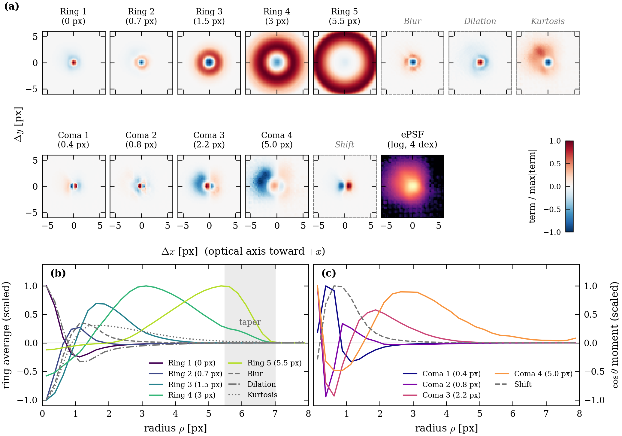
- The model. The radial shift with ring and coma basis functions (above) reproduces the shift to within 0.6 mpx: the shift left in the residual is $+0.2$ to $+0.6$ mpx, largest for S23 C4 K2 ($+0.6\pm0.2$ mpx, 3$\sigma$) and within 1$\sigma$ elsewhere (Table 4; means over one outlier-clipped star set, so data = model + residual exactly). Fig. 12 shows the basis functions.
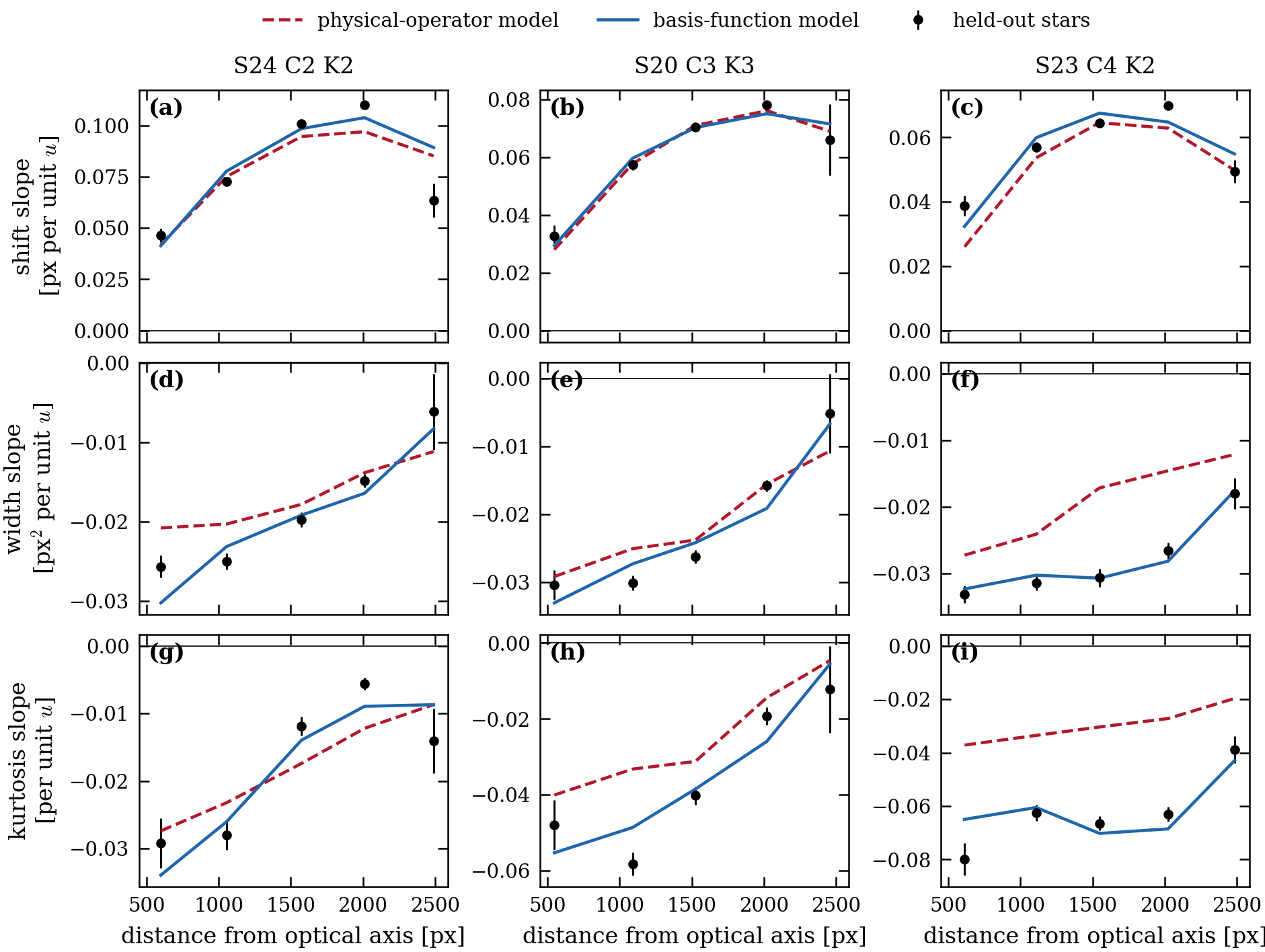
- Physical comparison. Against the data, the basis-function model's width and kurtosis slopes follow the data in physical terms (Fig. 13). The earlier physical-operator model, which moves core and wing in fixed ratios, is compared in Appendix D.
- Limit. A red core residual remains inside about 1.3 px; faint stars ($T>13$) are out of scope.
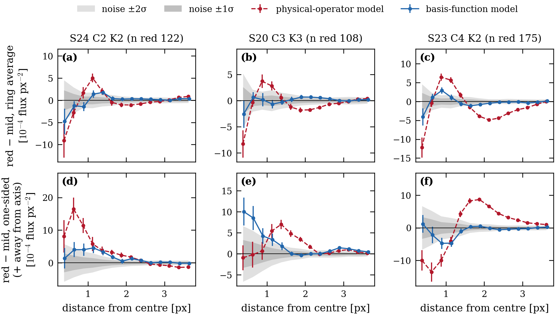
The two colour models compared with the data in physical terms, on held-out stars of three fields, each model fitted to the same preliminary image with the same folds (folds 0 and 1 of each field). (a–i) Colour slope (per unit $u$, a straight line over $0.4<u<1.8$) of radial shift, $\Delta W$ and $\kappa$ against distance from the optical axis. Points: held-out stars with bootstrap errors; lines: the same per-star estimator applied to each model's rendered image (dashed red: physical-operator model; solid blue: basis-function model). Both models reproduce the shift. The operator model's width and kurtosis slopes are too shallow, by about a factor of two on S23 C4 K2 (data/model slope ratio 1.2–1.8 in width and 1.9–2.3 in kurtosis); the basis-function model follows the data (ratio 0.92–1.23 there). Supplement (a–f): held-out $T=10$–13 red minus mid-colour residual (data − model, per unit flux), ring average (a–c) and one-sided component along the axis direction (d–f, positive away from the axis), against distance from the star centre; grey bands: ±1σ and ±2σ noise from disjoint halves of the mid-colour stars. The operator model leaves structure out to 2.5–3 px in every field (up to $-14\times10^{-4}$ one-sided on S23 C4 K2); the basis-function model is inside the noise beyond about 1.3 px. Inside 1 px it leaves a red one-sided core residual on S20 C3 K3 ($+10$ and $+8.5\times10^{-4}$ in the two innermost bins, outside the ±2σ band) that the operator model does not; on the other two fields its core residual is the smaller one.
Images behind it: red minus mid-colour residual profiles
4.6 Brightness dependence
The adopted model has one ePSF for all brightnesses and no brightness term. The brightness dependence is not fitted but measured, from the held-out residuals of the fit (below). A linear peak-charge width term that we tested, and why it is not adopted, is in Appendix E.
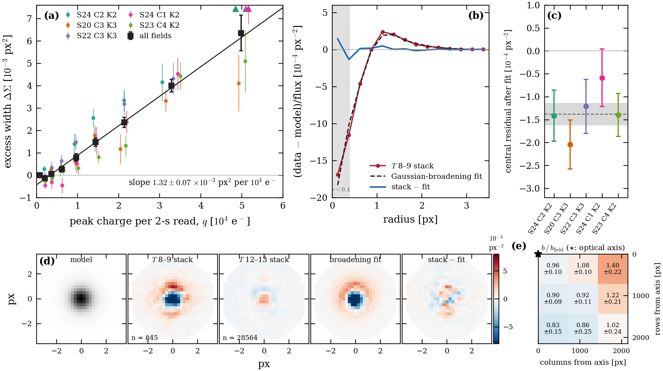
Suppose that, for a group of stars, the true PSF is the model $P$ blurred by an isotropic Gaussian of variance $\Delta\Sigma$ per axis. The stacked residual divided by flux is then $$\frac{\text{data}-\text{model}}{f}\simeq\tfrac12\,\Delta\Sigma\left(\partial_x^2P+\partial_y^2P\right),$$ where $f$ is the star's flux, $P$ the unit-flux model image (px$^{-2}$) and $\Delta\Sigma$ (px$^2$) the excess width, positive when the data are broader than the model. We fit each stack on held-out stars, together with flux, centroid and background terms, and use the peak charge in one 2-s read, $q=2\,{\rm s}\times f\times\phi$, as the brightness variable ($\phi$ is the fraction of the flux in the brightest pixel; $q\approx6\times10^4$ e$^-$ at $T=8$).
- The width grows linearly with peak charge: pooled over five fields, $d\Delta\Sigma/dq=(1.32\pm0.07)\times10^{-3}$ px$^2$ per $10^4$ e$^-$ ($\chi^2=1.4$ for 6 degrees of freedom), zero below $q\approx3\times10^3$ e$^-$ ($T\gtrsim10.5$). The sign is the same in every field; the slope ranges from 1.06 to 1.62.
- At $T=8$–9 a Gaussian-broadening fit to the stack of 845 held-out stars gives $\Delta\Sigma=2.8\times10^{-3}$ px$^2$ relative to the model, about 0.2 % in the core width. The absolute scale of $\Delta\Sigma$ has a 10–15 % systematic uncertainty from the calibration of the measurement.
- A Gaussian broadening explains 87 % of the power of the bright stack within 3.5 px. What remains is small but not noise.
- The effect resembles the brighter-fatter effect of CCDs (Antilogus et al. 2014; Guyonnet et al. 2015): charge already collected in a pixel deflects later photo-electrons toward its neighbours.
- Leaving it out costs little: adding a width term lowers the held-out $\chi^2$ by 1.2 % at $T=8$–10.5 and 0.12 % at $T=10.5$–13, and changes PSF magnitudes by between $-0.45$ mmag ($T\approx8.25$) and $+0.19$ mmag ($T\approx12.75$) (Appendix E).
Excess PSF width relative to the adopted model, measured on held-out stars in five fields. (a) Excess width $\Delta\Sigma$ against peak charge $q$ per 2-s read, relative to each field's faint stars; coloured points are fields, black squares the weighted mean, the line a straight-line fit with the slope given. (b) Azimuthal profile of the pooled $T=8$–9 stack, its Gaussian-broadening fit and the remainder. (c) Central residual after the same fit, per field. (d) Model image, stacked residuals at $T=8$–9 and $12$–13, the broadening fit and the remainder, on one colour scale ($10^{-4}$ px$^{-2}$). (e) Field-normalised per-star coefficient $b/b_{\rm field}$ in a $3\times3$ grid over the CCD, by distance from the optical axis (star). Triangles at the top of (a) mark three field points at $q\approx5\times10^4$ e$^-$ that lie above the plotted range (8.5–16.6, in the same units).
4.7 What remains
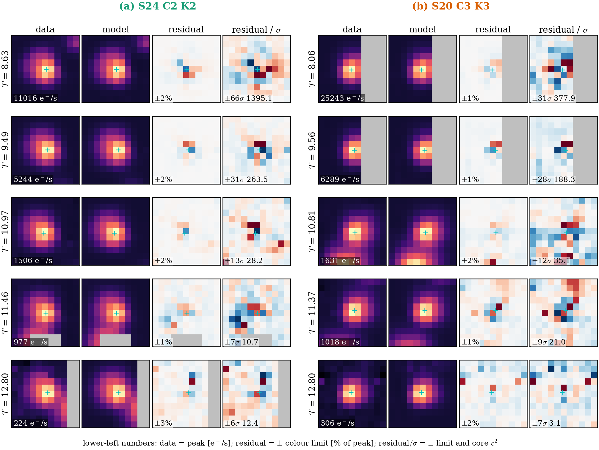
- Held-out stars are reproduced pixel by pixel to a few per cent of the peak (Fig. 15, stamps). Residuals at the bright end are a small, structured central pattern (score images).
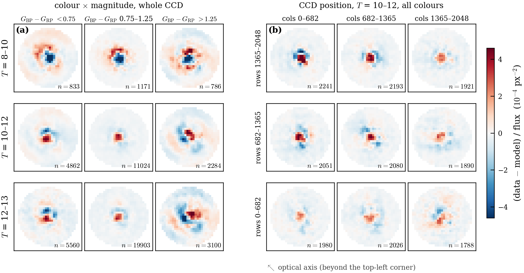
- The median held-out $c^2$ per pixel falls from about 500 at $T=8$–9 to about 6 at $T=12$–13, and the held-out to in-training ratio is 1.2–1.3 at $T=8$–9 (Table 3).
- The colour terms lower the $c^2$ at every brightness (Table 4).
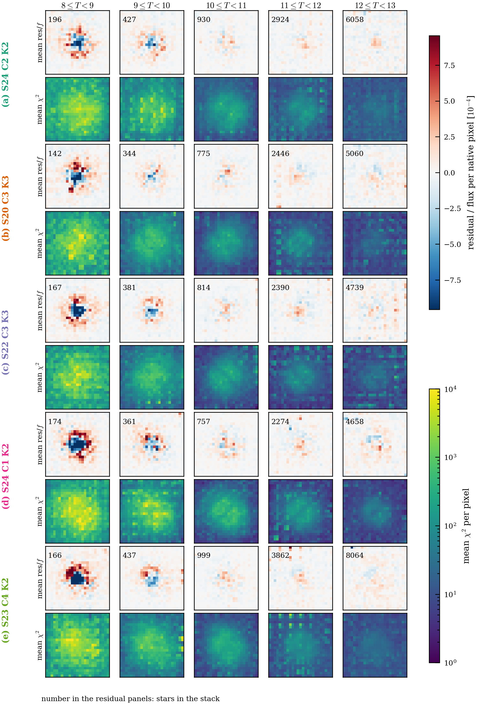
Stacked held-out residuals, (data − model)/flux, of 49,529 stars from the fit to the preliminary image, five fields pooled (CCD 3 mirrored so that the optical axis lies beyond the top-left corner in every field); 5σ-clipped means on one symmetric colour scale (±4.6×10$^{-4}$ px$^{-2}$; the brightest cores saturate), with the star count in each tile. (a) TESS magnitude (rows) against $G_{\rm BP}-G_{\rm RP}$ colour (columns), over the whole CCD. (b) Position on the CCD in a $3\times3$ grid, for $T=10$–12 and all colours. The brightest stars ($T=8$–10) keep a central deficit with a surrounding ring, the brightness effect of §4.6. Blue and red stars keep dipoles of opposite sign at every magnitude, while mid-colour stars leave only a small central excess. The central excess at $T=10$–12 is largest near the optical axis (about $7\times10^{-4}$) and smallest at the far corner (about $3\times10^{-4}$).
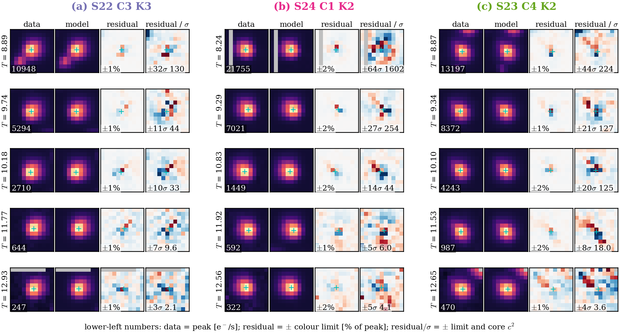
Held-out stars of F1 (left) and F2 (right) nearest the CCD centre in each magnitude bin ($T=8$ to 13). Columns: data, model, residual (shared scale as a percentage of the peak) and residual in units of the noise. The cross marks the fitted position, grey pixels are masked, and $c^2$ is the mean $\chi^2$ per pixel within the star's core ($r\le3$ px), $\chi^2=(D_p-m_p)^2/\sigma_p^2$.
Other fields (S22, C1, C4)
(a) Median core $c^2$ per pixel against $T$, held-out (solid) and in training (dashed), for five fields. (b) Held-out over in-training ratio. (c) Median held-out $c^2$ against colour offset. (d, e) Learning curves of the held-out median $c^2$ for the shape and colour stages. (f) Fractional decrease of the training loss per step against the stop-rule tolerance.
Mean held-out residual divided by flux (top rows, shared colour scale) and mean $\chi^2$ per pixel (bottom rows) for stars of five magnitude bins in each field, with the number of stars. At $T=8$–9 a central deficit with a positive ring is visible in every field; it is the brightness effect of §4.6. Fainter bins show only weak structure.
For each field: held-out cores, colour range, WCS bias and scatter against the FFI header WCS on the same stars, median core $c^2$ in three magnitude bins, held-out over in-training ratio at $T=8$–9, and the photometric scatter and colour slope against Gaia-XP (§5.5).
| FFI | held-out cores | colour $u-u_{\rm ref}$ 5–95% | WCS bias x, y [mpx] | WCS σ x, y [mpx] | header WCS σ x, y [mpx] | median $c^2$ T8–9 / 10–11 / 12–13 | held/in-training T8–9 | Δm σ T10–12 [mmag] | Δm colour slope [mmag/mag] |
|---|---|---|---|---|---|---|---|---|---|
| S24 C2 K2 | 10,536 | -0.31 … +0.49 | -0.2, +0.2 | 6.2, 4.9 | 24, 31 | 505 / 43 / 6.4 | 1.2 | 12.0 | +37 ± 1 |
| S20 C3 K3 | 8,767 | -0.31 … +0.51 | +0.0, -0.1 | 4.5, 4.9 | 23, 26 | 461 / 36 / 4.1 | 1.3 | 12.0 | +35 ± 1 |
| S22 C3 K3 | 8,491 | -0.30 … +0.49 | -0.0, -0.0 | 4.9, 5.2 | 19, 24 | 488 / 38 / 4.1 | 1.3 | 11.6 | +36 ± 1 |
| S24 C1 K2 | 8,224 | -0.31 … +0.53 | -0.6, -0.3 | 7.3, 5.9 | 20, 16 | 797 / 62 / 6.4 | 1.2 | 12.6 | +40 ± 1 |
| S23 C4 K2 | 13,528 | -0.32 … +0.47 | +0.0, +0.0 | 5.1, 5.0 | 27, 20 | 671 / 52 / 6.1 | 1.2 | 14.3 | +38 ± 1 |
Red minus blue radial shift of $T=10$–13 stars, measured and modelled, the remaining difference, and the median held-out $c^2$ with the colour terms off and with the adopted model, in three magnitude bins.
| FFI | red − blue radial shift, measured [mpx] | model [mpx] | remaining [mpx] | $c^2$ colour-off / adopted, T8–9 / 10–11 / 12–13 | all held-out |
|---|---|---|---|---|---|
| F1 S24 C2K2 | -64.8 | -62.3 | +0.2 ± 0.4 | 5.07 / 3.55 / 1.80 | 2.19 |
| F2 S20 C3K3 | -48.4 | -46.6 | -0.3 ± 0.3 | 4.84 / 3.53 / 1.76 | 2.11 |
| S22 C3K3 | -51.8 | -50.2 | -0.3 ± 0.3 | 5.13 / 3.00 / 1.68 | 1.97 |
| C1 S24 C1K2 | -53.1 | -49.6 | -0.3 ± 0.5 | 3.16 / 2.26 / 1.61 | 1.81 |
| C4 S23 C4K2 | -40.1 | -38.6 | +0.7 ± 0.2 | 4.69 / 2.83 / 1.49 | 1.72 |
5 Final de-crowded image
§5.1 builds the final de-crowded image from the joint fit; §5.2–5.5 check it (image quality and colour residuals, refit stability, astrometry, bright-star photometry), and §5.6 uses it for targeted faint-star photometry.
5.1 Production with per-band kernels
- For each PS1 band we evaluate the fitted ePSF at that band's colour and remove the smoothing already applied to the template, giving a kernel $K_b$ at every position. Each calibrated band template is convolved with its own kernel and the sum is subtracted from the background-corrected FFI: $$D_{\rm final}=(I-B)-\sum_b K_b\ast f_{s,b}\,T'_b .$$ Here $T'_b$ is the band template rebuilt on the fitted WCS, $f_{s,b}$ its calibration factor in skycell $s$ (§2.5), and $K_b$ the band-$b$ kernel.
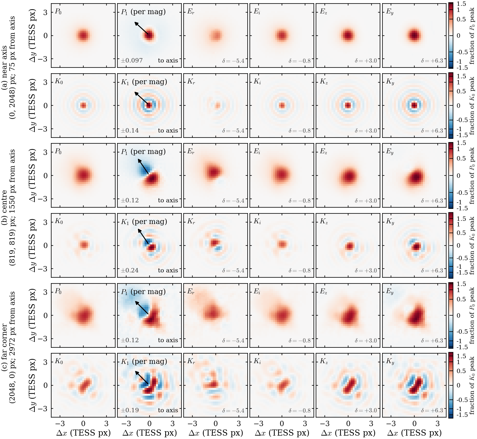
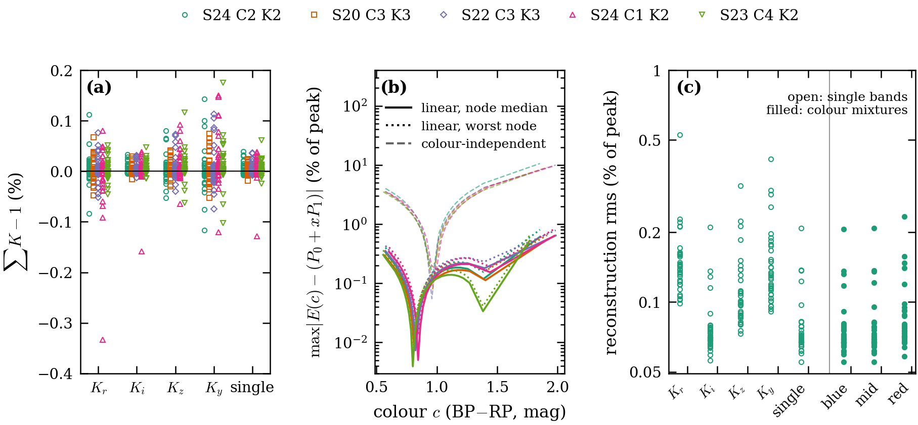
Kernels in S24 C2 K2 at three ePSF nodes: (a) near the optical axis (75 px from it), (b) the CCD centre (1550 px) and (c) the far corner (2970 px). Upper row of each pair: the ePSF linearised in colour, $E(c)\approx P_0+xP_1$, where $x=c-c_{\rm ref}$ is the star's colour offset from the reference colour ($G_{\rm BP}-G_{\rm RP}$, mag), $P_0$ the ePSF at the reference colour and $P_1$ its colour slope (per mag; the arrow points to the optical axis); and the band responses $E_b=P_0+\delta_bP_1$, with $\delta_b$ the effective colour offset of PS1 band $b$ ($-5.4$, $-0.8$, $+3.0$ and $+6.3$ mag for $r,i,z,y$). Lower row: the matching kernels $K_0$, $K_1$ and $K_b=K_0+\delta_bK_1$, which turn the Gaussian-smoothed template into $E_b$. Responses are scaled to the node's $P_0$ peak and kernels to its $K_0$ peak (asinh, linear within 25 % of the maximum); $P_1$ and $K_1$ have their own symmetric scales (the ± value in each panel). Redder bands are more peaked ($E_y$ peak 1.5–1.6 times the $P_0$ peak, against 0.5–1.1 for $E_r$). Near the axis the kernels are compact and round; toward the corner they become elongated, and the colour slope becomes a dipole along the axis direction of 10–12 % of the peak per mag. Supplement (kernel checks): (a) Sum of each kernel minus one, for the 36 nodes and four bands and for the single colour-independent kernel, five fields: within 0.18 % for every node but one ($-0.33$ %, S24 C1 K2). (b) Error of the linear colour expansion, the maximum of $|E(c)-(P_0+xP_1)|$ over the node as a percentage of its peak, against colour over the 2–98 % range of the training stars: node median (solid) and worst node (dotted), against the error of a single colour-independent ePSF (dashed). The median is 0.09–0.13 % and the worst 0.64–0.83 %, largest at the red end; a colour-independent ePSF errs by 1.5–1.8 % (median) and up to 8–13 %. (c) S24 C2 K2: a point source in the smoothed template, convolved with the kernel and summed to native pixels, minus $E_b$ rendered at the same sub-pixel position; rms over $23\times23$ px and $16\times16$ positions as a percentage of the native peak, one point per node. Open: single bands (median 0.07–0.14 %, at most 0.53 %); filled: the mixtures $K_0+xK_1$ at the 2, 50 and 98 % training colours, the kernels real stars see (median 0.07–0.08 %, at most 0.23 %).
Kernel checks
5.2 Image quality and colour residuals
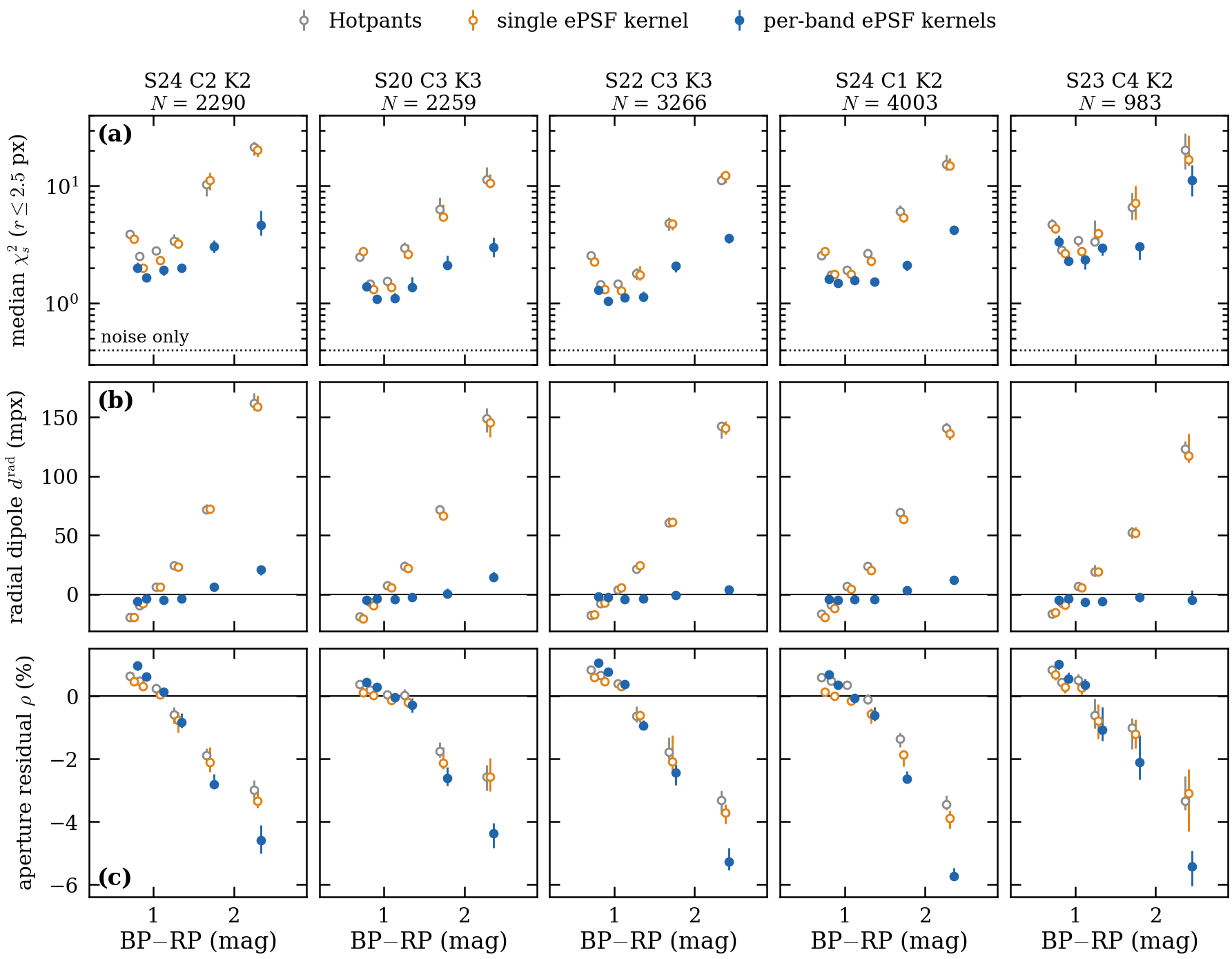
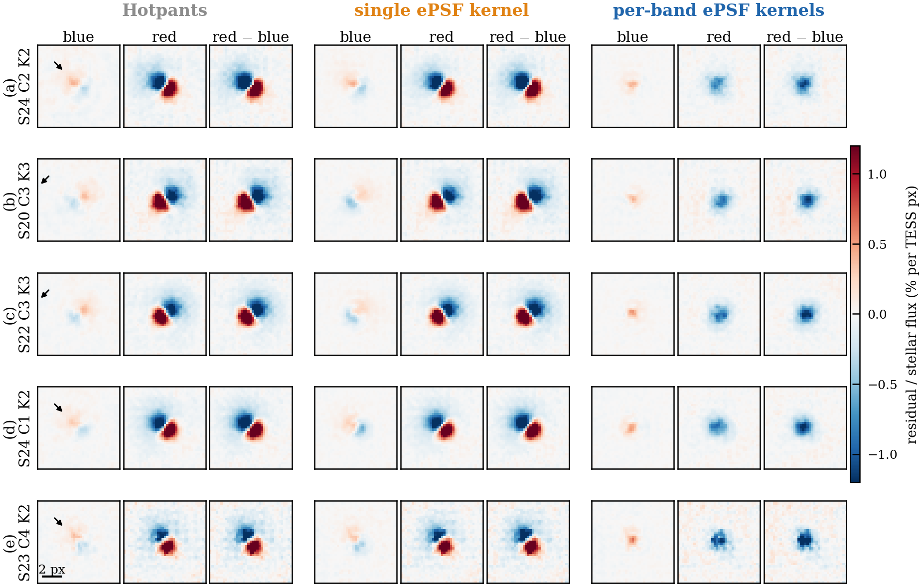
- On held-out faint stars ($13\le T<16$) the per-band kernels give the lowest core $\chi^2$ in every colour bin and remove the colour-dependent radial dipole that a single empirical kernel and a colour-independent kernel both leave (between the reddest and bluest colour bins, $+132$ to $+181$ mpx with the empirical and colour-independent kernels against $0$ to $+27$ mpx with the per-band kernels; the scorer's red−blue dipole for the per-band image is $+2$ to $+17$ mpx; reddest-bin $\chi^2$ lower by a factor of 2–4.5).
- The PS1 stack images are offset from their header WCS by about 0.1 arcsec relative to Gaia (the PS1 mean catalogue agrees with Gaia). Correcting the kernel position for this offset (with proper motion) and calibrating the band templates (§2.5) act together on an achromatic dipole of mid-colour stars: the shift corrects the stacks' astrometric offset and the calibration the per-band zero-point error. The shift alone halves it in S24 C2 K2 (10.6 to 4.9 mpx) but increases it in S20 C3 K3 and S22 C3 K3 (2.5 to 6.9 and 4.8 to 7.1 mpx), where the stack offset was not the dominant term. With both steps it is 0.8, 3.2, 2.0, 5.4 and 5.5 mpx in the five fields (before: 10.6, 2.5, 4.8, 13.0 and 10.3 mpx). Hotpants gives 0.5–1.7 mpx here because its kernel is fitted to stars of this colour. The residual of about 5 mpx in S24 C1 K2 and S23 C4 K2 is not explained.
- The PS1 template calibration (§2.5) removes about 4–5 mpx of a colour-independent radial offset (mid-colour stars move from $-7$ to $-9$ mpx to $-3$ to $-5$ mpx), so every colour bin shifts by the same amount; the red−blue dipole itself is unchanged by it (scorer metric changes $\le0.9$ mpx against uncertainties of 1.6–3.5 mpx). The colour-correct kernels expose a template excess for red stars (aperture residual $-4.4$ to $-5.7$ % for the reddest stars, against $-2.6$ to $-3.9$ % with the empirical and colour-independent kernels): the template over-predicts the TESS flux of red stars. The band synthesis is ruled out (the template follows Gaia-XP colour to $\le0.4$ % per mag), and §6 discusses the origin.
Held-out faint stars ($13\le T<16$) on identical templates, WCS and stars, for three subtractions: Hotpants (one empirical kernel), a single colour-independent ePSF kernel, and per-band kernels from the chromatic ePSF. Rows: median core $\chi^2$ within 2.5 px; radial residual dipole (mpx, positive away from the optical axis); and aperture residual, the fraction of the star's flux left within 3.5 px (negative means over-subtraction). The per-band kernels give the lowest $\chi^2$ in every colour bin and remove the colour-dependent dipole, leaving a constant radial offset of about $-8$ mpx that comes from the template colour zero point. The reddest stars have the most negative aperture residual (about $-5$ to $-6$ %), the sign of a template that is too bright for red stars. In (c) the per-band image leaves the MOST negative aperture residual for the reddest stars ($-4.4$ to $-5.7$ %, against $-2.6$ to $-3.9$ % for Hotpants and the single kernel): the colour-correct kernels expose the template's red excess, which the empirical kernels partly absorb. Its origin is discussed in §6 (red total-flux deficit) and Appendix F.
Images behind it: stacked residuals by colour
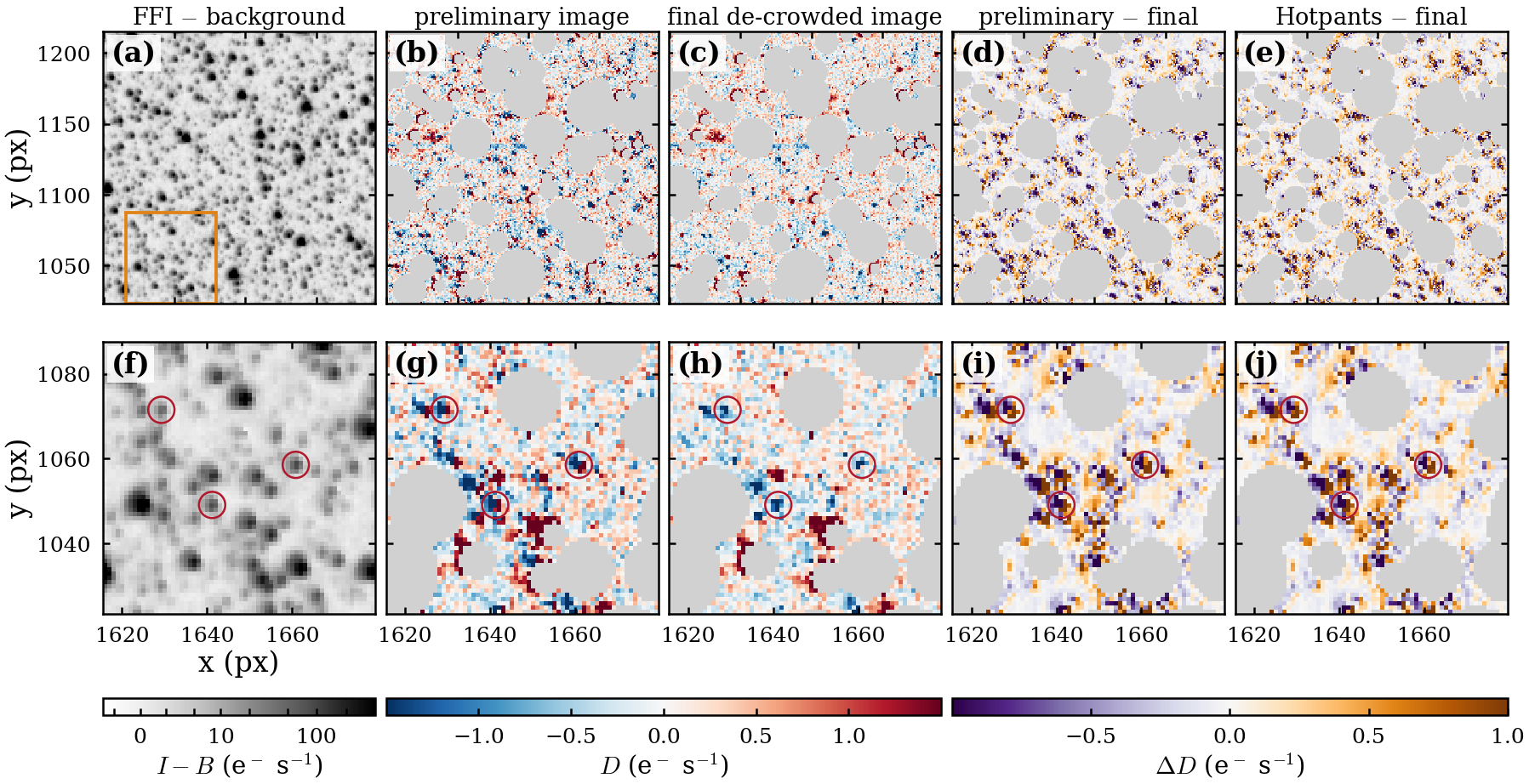
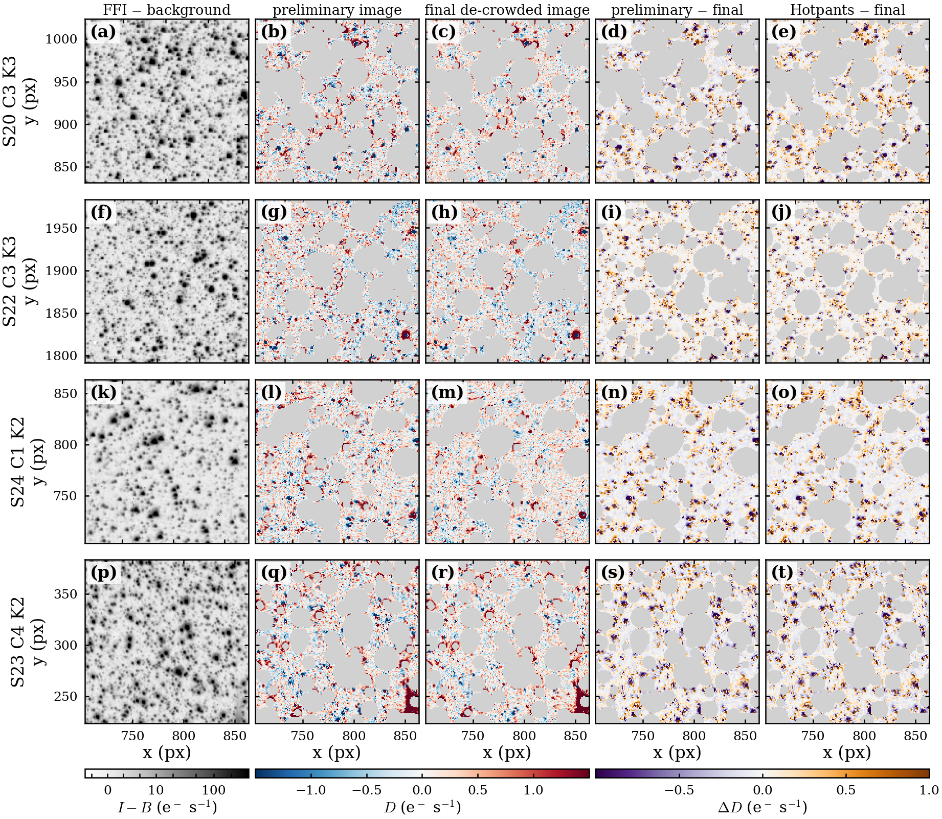
A $192\times192$-px region of S24 C2 K2 ($x$ 1600–1792, $y$ 1024–1216; top) and a $64\times64$-px zoom (orange box in a; bottom), the sub-tile with the most red held-out stars. Columns: (a, f) FFI minus background; (b, g) the preliminary de-crowded image (§3); (c, h) the final de-crowded image (§5.1); (d, i) preliminary minus final; (e, j) Hotpants with one empirical kernel on the same final template, minus final. Grey: footprints of the $T\le13$ stars (radius $3+3(13-T)$ px, at most 40 px), which are not in the template and keep their full flux in every image. Circles: red ($G_{\rm BP}-G_{\rm RP}\ge1.5$) held-out stars used to score the images. Outside the footprints the robust scatter of $D$ is 0.46 e$^-$ s$^{-1}$ in the preliminary image, 0.39 in the final image and 0.46 with Hotpants, and the fraction of pixels beyond $5\sigma$ falls from 2.0 % to 1.0 % ($\sigma$ from the Hotpants noise plane, which overestimates the noise by about 1.6 times). The residuals at the red stars are weaker in the final image. The two difference images are nearly the same (rms 0.73 e$^-$ s$^{-1}$ each). One colour scale per quantity, shared by all region figures. Supplement (other fields): The same for the other four fields, one row each: S20 C3 K3 ($x$ 256–448, $y$ 832–1024), S22 C3 K3 (1216–1408, 1792–1984), S24 C1 K2 (1664–1824, 704–864) and S23 C4 K2 (704–864, 224–384); $x$ ticks are labelled for the bottom row only. Outside the footprints the robust scatter of $D$ falls from 0.42–0.49 e$^-$ s$^{-1}$ in the preliminary image (and with Hotpants) to 0.38–0.43 in the final image, and the fraction of pixels beyond $5\sigma$ from 1.5–2.4 % to 0.9–1.9 %. The bright residual at the lower right of (q, r) is common to both images.
Other fields
(a) For each PS1 skycell covering S24 C2 K2, the offset $\Delta\boldsymbol\alpha$ of the light in the stack image from the position its header WCS predicts, measured on isolated Gaia stars ($14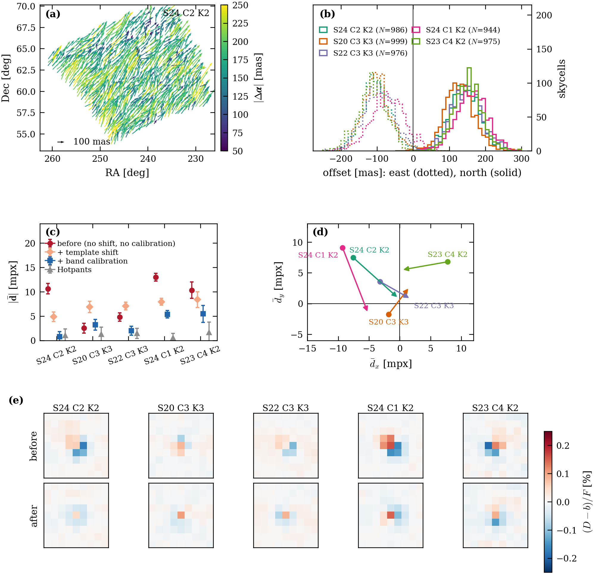
5.3 Refit stability
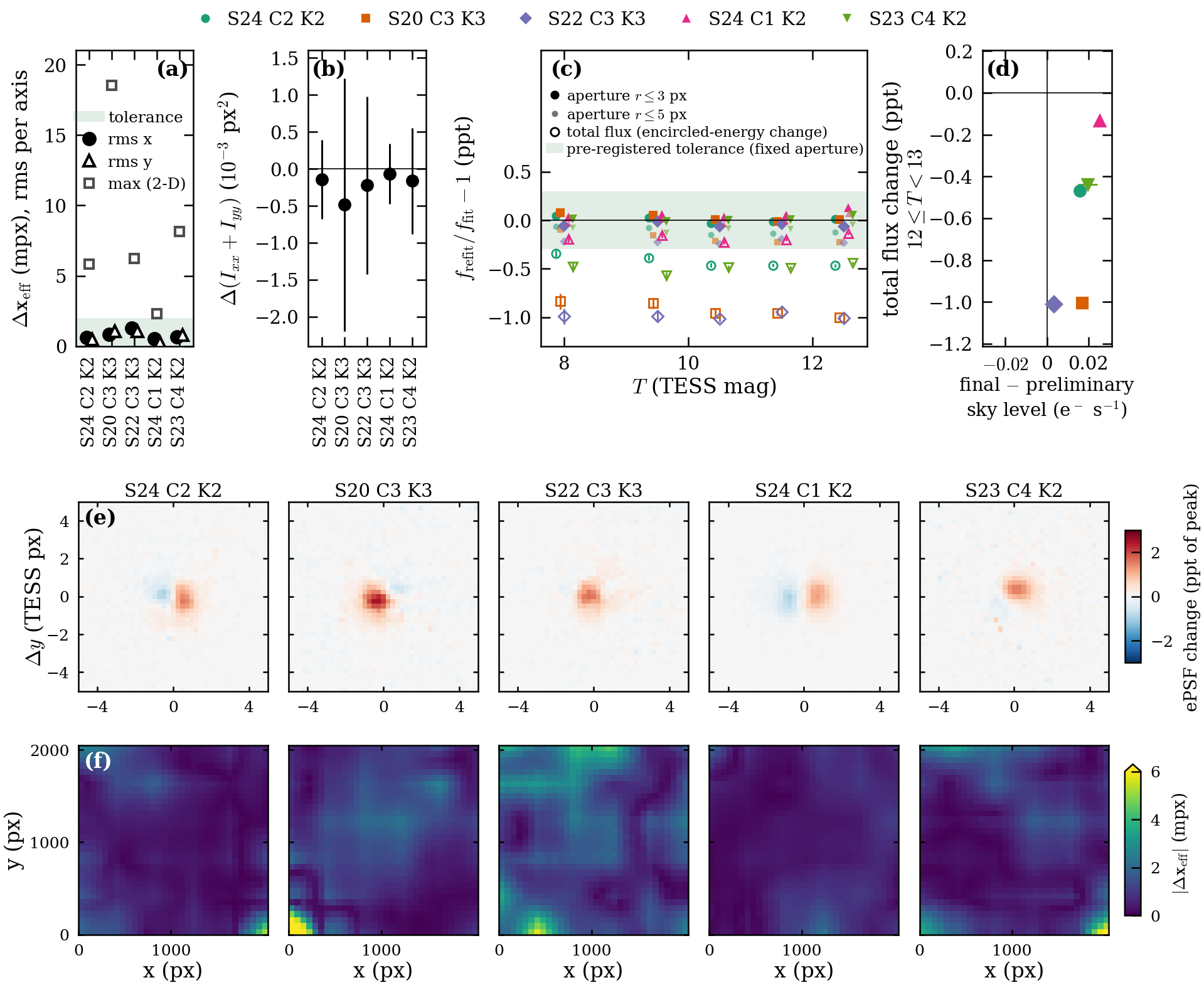
- We refit the joint model on the final de-crowded image and compare with the fit on the preliminary image, with pre-registered tolerances of 2 mpx rms per axis in effective star position and 0.3 ppt per magnitude bin in the flux within fixed apertures of 3 and 5 px radius. A further check asks that the held-out $\chi^2$ of the refit be no larger than that of the preliminary-image fit in each magnitude bin.
- Position: all five fields pass, 0.25–1.29 mpx rms per axis (largest S22, 1.29 and 1.06 mpx). In S22 the WCS change (3.3 mpx rms) and the ePSF-centroid change are each large and nearly opposite, so they largely cancel; we attribute the remaining few-mpx structure across the CCD, as an untested hypothesis, to S22's preliminary image changing most with the background.
- Flux: the gate quantity is the flux within fixed apertures of 3 and 5 px radius, with a pre-registered tolerance of 0.3 ppt per magnitude bin. All five fields pass, with at most 0.13 ppt ($r\le3$ px) and 0.24 ppt ($r\le5$ px). The total model flux changes by $-0.1$ to $-1.0$ ppt (at $12\le T<13$: S24 C1 K2 $-0.13$, S23 C4 K2 $-0.44$, S24 C2 K2 $-0.47$, S20 C3 K3 $-1.00$, S22 C3 K3 $-1.01$). It is flat in $T$ and equals the change of the ePSF's encircled energy within 3 px, so it is light moved between core and wing.
- ePSF size: the median change of the second-moment size over the nodes is $-0.06$ to $-0.16\times10^{-3}$ px$^2$ in S24 C1 K2, S24 C2 K2 and S23 C4 K2 (within $\pm0.2\times10^{-3}$ px$^2$), $-0.22\times10^{-3}$ px$^2$ in S22 C3 K3 and $-0.49\times10^{-3}$ px$^2$ in S20 C3 K3. The node-to-node scatter of the change is 0.4–1.7$\times10^{-3}$ px$^2$ in every field. No tolerance was set for this quantity.
- Held-out $\chi^2$: the refit is no worse in all five magnitude bins in S24 C2 K2, S22 C3 K3 and S24 C1 K2. In S23 C4 K2 it is no worse in four bins; the exception is $T=8$–9, at a ratio of 1.003, within the noise. In S20 C3 K3 it is no worse in three bins; at $T=8$–9 and 9–10 the refit is worse by 10 % and 2 %, which we accept.
- Memorisation limit: at $T=8$–9 the held-out $\chi^2$ exceeds the in-training $\chi^2$ by a factor 1.09–1.40 (median over folds, per field; single folds up to 1.83), on both the preliminary and the final image. The pre-registered check on this ratio is therefore not met in any field. The ePSF partly memorises its brightest training stars, a limit of fitting a single image.
- Sky: the offset between the preliminary and final subtractions is 0.003–0.025 e$^-$ s$^{-1}$ in all fields and does not correlate with the total-flux change, so the total-flux change is a redistribution of ePSF light between core and wing, not a sky effect.
Refit on the final de-crowded image minus the fit on the preliminary image, five fields. (a) Effective star-position change (WCS plus ePSF centroid), rms per axis over held-out stars, against the pre-registered 2 mpx tolerance (shaded); all five fields pass (0.25–1.29 mpx; largest S22, 1.29 and 1.06 mpx). Open squares give the largest per-star change $|\Delta\boldsymbol x_{\rm eff}|$ over all fitted stars ($T\le13$); it is 2–8 mpx in four fields and reaches 18.5 mpx in S20 C3 K3, at the bottom-left corner of the CCD where (f) saturates, and is not part of the tolerance, which is set on the rms. (b) Change of the ePSF second-moment size $\Delta(I_{xx}+I_{yy})$ in $10^{-3}$ px$^2$, median over the nodes with the node-to-node rms as the bar (no tolerance was set for this quantity). (c) Flux change $f_{\rm refit}/f_{\rm prelim}-1$ in ppt against $T$, per magnitude bin. Filled: flux within fixed apertures of 3 px (large) and 5 px (small) radius, the gate quantity, with its pre-registered tolerance of 0.3 ppt (shaded); every field passes (at most 0.24 ppt). Open: total model flux, $-0.13$ to $-1.01$ ppt and flat in $T$. It has no tolerance, because it equals the change of the ePSF's encircled energy within 3 px, i.e. light moved between core and wing. (d) Sky offset of the final minus preliminary subtraction (0.003–0.025 e$^-$ s$^{-1}$) against the total-flux change at $12\le T<13$, which do not correlate. (e) Change of the ePSF averaged over the nodes, in ppt of the peak, one colour scale. (f) Median $|\Delta\boldsymbol x_{\rm eff}|$ of the fitted stars in 64-px cells over the CCD.
5.4 Astrometry
- These positions come from the joint fit on the preliminary image, scored on held-out stars. The refit on the final image moves positions by only 0.25–1.29 mpx rms (§5.3), so they hold for the final image.
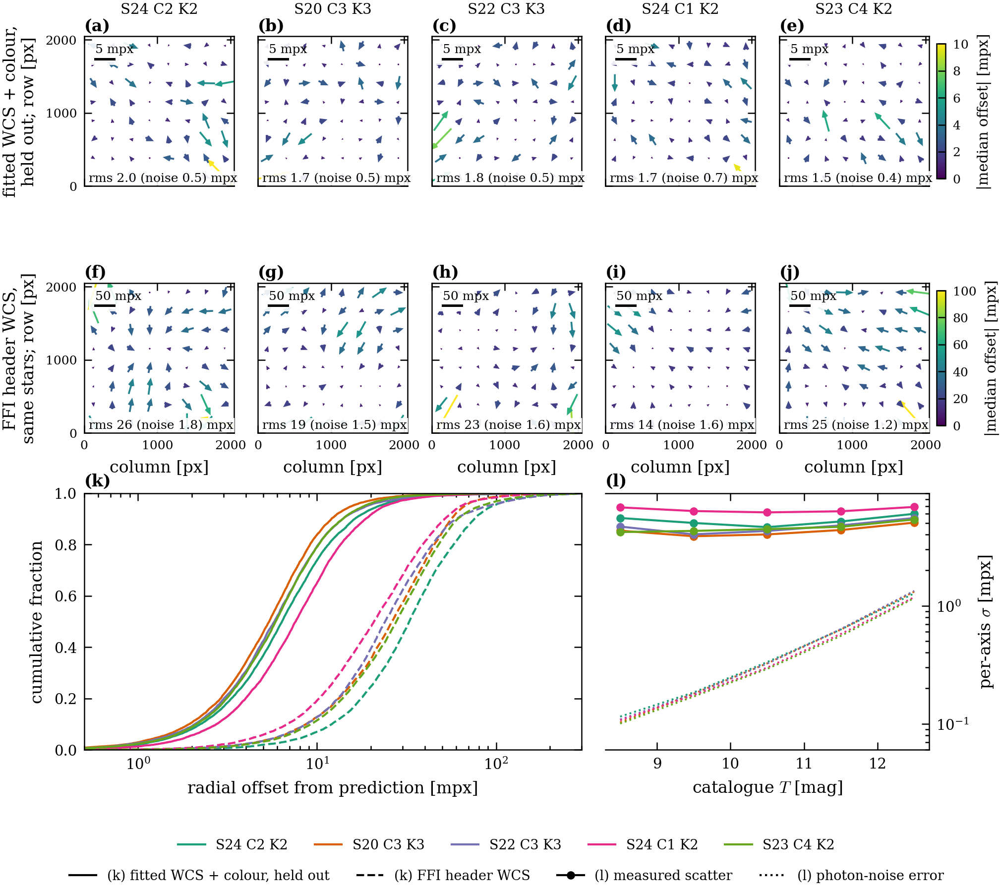
- Held-out stars, scored with the fits that did not use them, have a per-axis position scatter of 4.5–7.3 mpx with the fitted WCS and colour model, against 16–31 mpx with the FFI header WCS on the same stars.
- The scatter is flat with magnitude while photon noise runs 0.1–1.3 mpx, so it is a systematic floor, not noise. Cell-median maps leave a coherent 1.5–2 mpx pattern, largest at the CCD edges and corners.
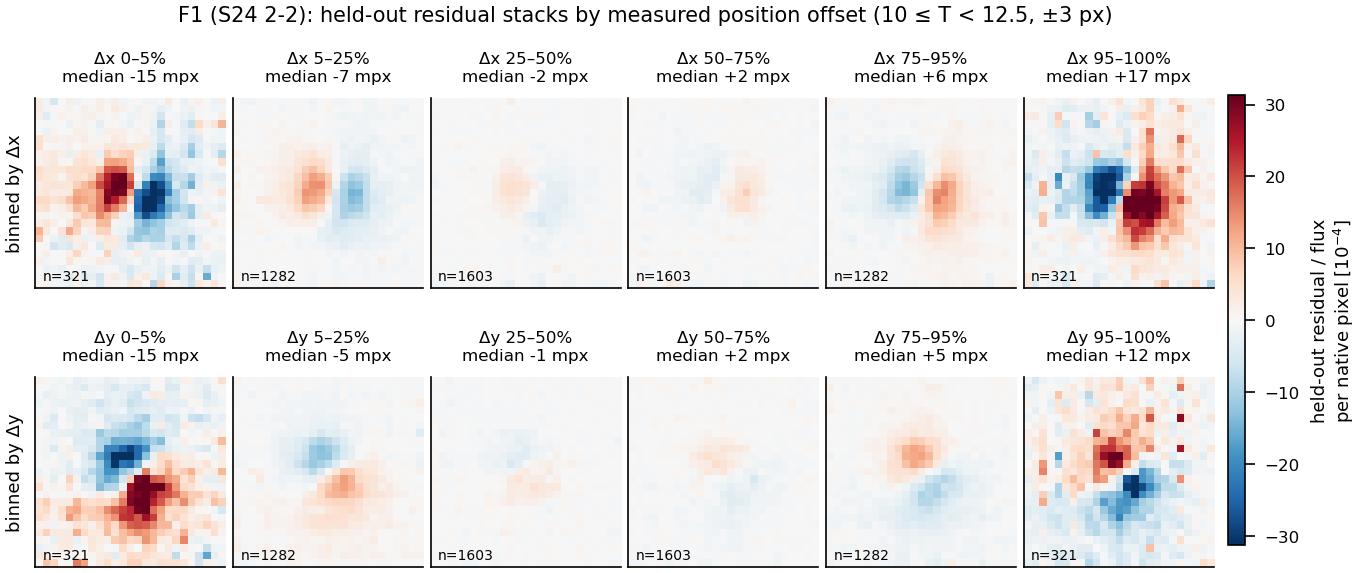
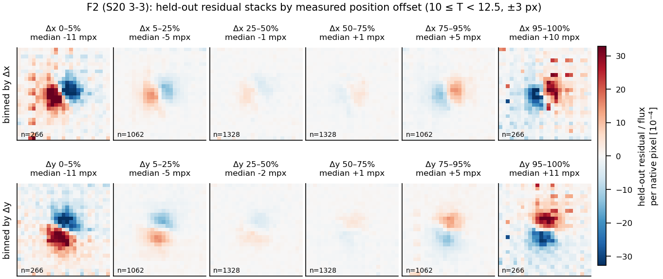
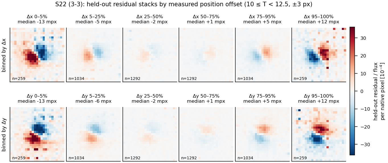
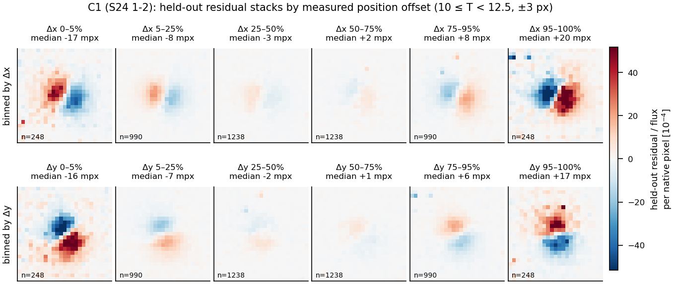
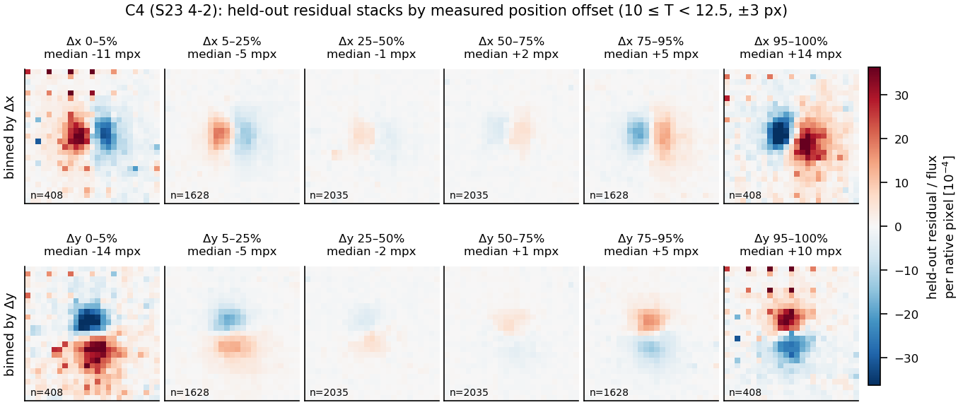
Top: cell-median position offsets of held-out stars with the fitted WCS and colour model (arrows, scale 5 mpx). Middle: the same stars with the FFI header WCS (scale 50 mpx). Bottom left: cumulative distribution of the radial offset with a constant offset removed. Bottom right: measured per-axis scatter against $T$, against the photon-noise error. The stacked residuals of stars binned by measured offset show clean dipoles whose sign follows the offset, so the offsets are real image shifts.
Images behind it: residual stacks binned by measured offset, per field
5.5 Bright-star photometry
- These fluxes come from the joint fit on the preliminary image, scored on held-out stars. The refit on the final image changes fixed-aperture fluxes by at most 0.24 ppt (§5.3), so they hold for the final image.
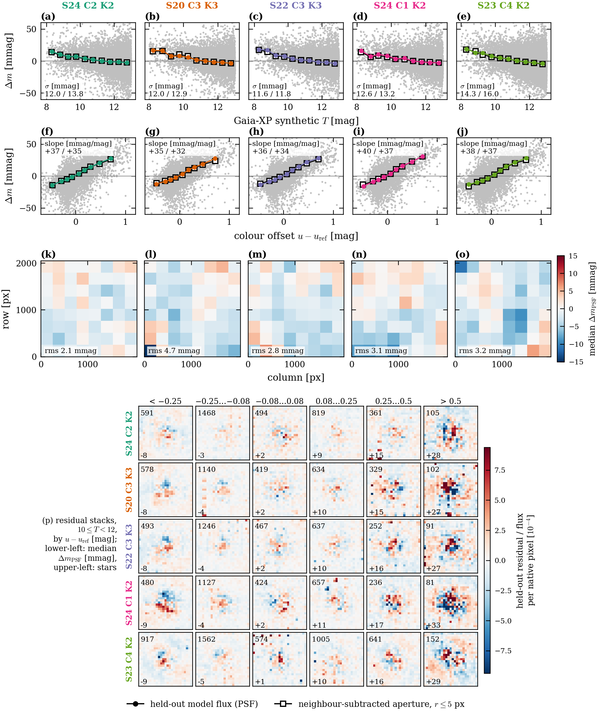
- Held-out PSF fluxes agree with Gaia-XP synthetic TESS magnitudes with a scatter of 11.6–14.3 mmag at $T=10$–12. Neighbour-subtracted aperture fluxes give a similar scatter, 11.8–16.0 mmag.
- Magnitude differences depend on colour with a slope of +35 to +40 mmag per mag of colour offset. This slope uses the colour offset $u-u_{\rm ref}$ and Gaia-XP spectra extended beyond 1020 nm with a power law; anchoring the red end to 2MASS $J$ and expressing the slope in $G_{\rm BP}-G_{\rm RP}$ gives the 25–30 mmag per mag of §6 (on the same stars the anchoring alone lowers it from 40.5 to 29.3 mmag per mag, so the extrapolated tail accounts for about a quarter).
- Held-out magnitudes run faint relative to Gaia-XP for the brightest stars: the pooled $\Delta m$ is $+15$ mmag at $T=8$–9 and $-3$ mmag at $T=12$–13, the same in all five fields. It appears equally with neighbour-subtracted apertures and does not change with aperture radius from 5 to 12 px, so it is not light outside the PSF model. About a third of the faint-end slope is a magnitude-dependent calibration error of the Gaia XP spectra: with the corrected XP spectra of Huang et al. (2024) the excess at $T=8$–9 drops to $+11$ mmag and the slope to about 2 mmag per mag. The remainder is not explained by any reference correction and is most likely on the TESS side; we report it as a limit of the absolute flux scale at the bright end.
- Held-out fluxes also depend weakly on where a star falls within a pixel: stars centred on a pixel are 1.5–2.5 mmag fainter than stars near a corner, mostly along columns. The dependence is the same for PSF and aperture fluxes and at all magnitudes, so it is a property of the detector's intra-pixel response that a single pixel-integrated ePSF cannot represent; it limits the flux accuracy at the $\le0.25$ % level.
Magnitude difference $\Delta m$ between held-out fluxes and Gaia-XP synthetic $T$ against $T$ (top row), against colour offset (second row; slopes in mmag per mag), as median maps over the CCD (third row; cell rms 2.1–4.7 mmag), and as residual stacks by colour bin (bottom). Circles are PSF fluxes, squares neighbour-subtracted aperture fluxes of radius 5 px. Held-out magnitudes run faint relative to Gaia-XP for the brightest stars, by about +15 mmag at $T\approx8.3$ falling to $-4$ mmag at $T\approx13$, identically in all five fields; this is a limit of the absolute flux scale at the bright end. Stars centred on a pixel are 1.5–2.5 mmag fainter than stars near a corner, a property of the detector's intra-pixel response that a pixel-integrated ePSF cannot represent.
5.6 Targeted de-crowding and faint-star photometry
- For a target star we take its own PS1 source segment in each band and push it through the same smoothing, resampling and kernels as the template, giving a modelled target image $M_t$ (Table 1, steps 14–15).
- Adding $M_t$ back to the final image, $D_t=D_{\rm final}+a\,M_t$, where $a$ is the smooth flux scale (second-order Chebyshev in position) fitted when the final image was made, restores the target's light so that its flux can be fitted together with its neighbours, while bright stars are measured directly on $D_{\rm final}$.
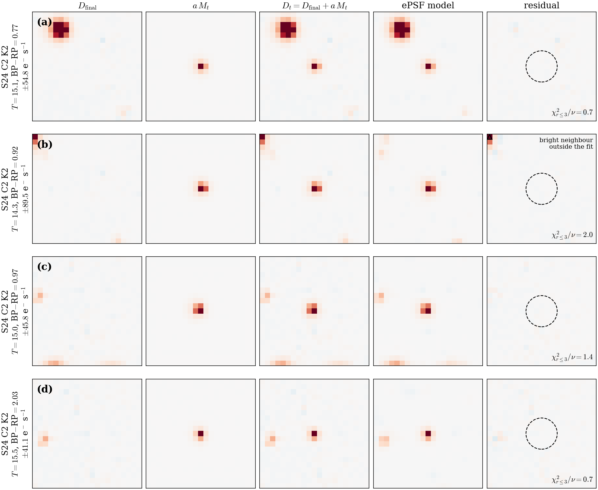
- Profiles and WCS are those fitted on the preliminary image; they are applied to the final image without refitting (Fig. 23: core $\chi^2/\nu$ within 3 px of 0.7–2.0 on four catalogue-selected targets).
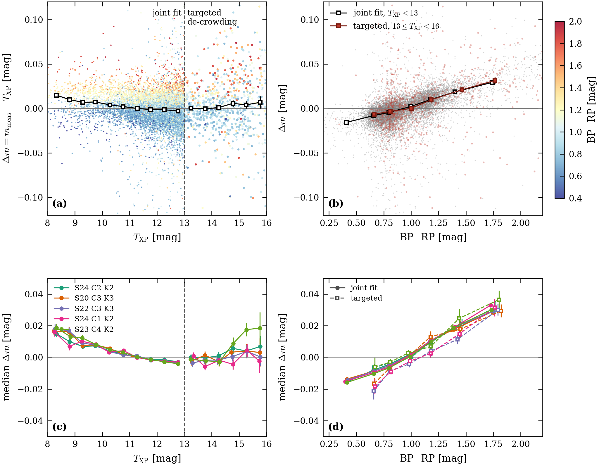
- Against Gaia-XP synthetic $T$ (Fig. 24) there is no step at $T=13$ between the joint-fit and the targeted fluxes ($-0.4$ to $+2.4$ mmag) in any field, and the faint colour slope (35–41 mmag/mag) matches the bright one (35–39 mmag/mag). The faint scatter grows from 14–21 mmag at $T=13$–13.5 to 37–65 mmag at $T=15.5$–16. The faint end of S23 C4 K2 rises by $+10$ to $+20$ mmag at $T=14.5$–16; the cause is not investigated.
Targeted de-crowding of four faint stars of S24 C2 K2. Columns: the final image with the target absent, the target's own template image (scaled to the image), their sum, the ePSF model (target, fitted neighbours and constant) and the residual. The colour scale is symmetric about zero and shared along each row (limit printed under the row label; set by the target's central 5×5 pixels, so neighbours saturate). The dashed circle is the $r=3$ px target aperture; $\chi^2_{r\leq3}/\nu$ is computed inside it (one free flux). Targets were chosen from the Gaia catalogue before any residual was examined: $14\le T<15.5$, no source $\ge1$ % of the target flux within 3 px, a source $\ge10$ % at 3–6 px, no $T<10$ star within 15 px; the first candidate by Gaia source_id in each of three colour bins (BP$-$RP $<0.8$, 0.8–1.4, $>1.4$; the middle bin twice) whose extraction succeeded. The $T<10$ cut was added after a first look at the stamps (it removes bleed trails; it uses the catalogue only). Row (b) has a bright neighbour at the stamp corner that is not part of the targeted fit. The ePSF and WCS are those fitted on the preliminary image, applied to the final image; the template image of each target is built with the same per-skycell calibration and kernels as the final image.
Photometric consistency with Gaia-XP synthetic T. (a,b) S24 C2 K2: joint-fit fluxes of held-out stars with $T_{\rm XP}<13$ (small points, open squares = medians) and targeted-extraction fluxes of $13\le T_{\rm XP}<16$ stars (large points, filled squares); zero point from the bright $10\le T_{\rm XP}<12$ stars; points coloured by BP$-$RP in (a). (c,d) medians for each field (filled: joint fit, open: targeted). The faint end of S23 C4 K2 rises to $+10$ to $+20$ mmag at $T=14.5$–16 (cause not investigated). Fluxes use the ePSF and WCS fitted on the preliminary image, applied to the final image. $T_{\rm XP}$ integrates Gaia-XP spectra extended beyond 1020 nm with a power law, and the colour is BP$-$RP, as in §5.5.
6 Discussion and limits
- Red total-flux deficit. We compare the total flux of isolated stars with the flux predicted from their Gaia DR3 XP spectra integrated through the TESS response function (version 2.0). Red stars are systematically fainter than predicted, by $b=25$–$30$ mmag per magnitude of $G_{\rm BP}-G_{\rm RP}$ ($+29\pm2$ mmag mag$^{-1}$ when the spectrum beyond 1000 nm is anchored to 2MASS $J$). The slope is consistent across all four cameras within 2–3$\sigma$ (per-field values 25–36 mmag mag$^{-1}$, driven by camera 1), and agrees on the same CCD in two sectors. It does not depend on brightness over $8\le T\le12.5$, and is seen independently in template-subtracted images of $13\le T\le16$ stars. Within small apertures the deficit is largely hidden: red stars are more centrally concentrated, which adds about as much flux at small radius as the total-flux deficit removes, so residuals within 3.5 px look consistent with version 2.0 (the colour slope relative to XP is close to zero at 2 px and $-3$ to $-3.5$ % per mag at 4–8 px). It is not light scattered outside the photometric aperture: the colour slope is constant from 6 to 150 pixels, less than 16 % (2$\sigma$) of the deficit can lie between 8 and 40 pixels, and less than 5 % lies in row or column streaks. It is not an error in the Gaia spectra: a prediction made without XP, by fitting model atmospheres to APASS and 2MASS photometry, also gives a positive slope (26–39 mmag mag$^{-1}$ depending on the atmosphere grid), and XP synthetic photometry agrees with Pan-STARRS1 $y$ to within 0.65 % per mag in all fields. The most likely explanation is that the in-flight red response of TESS is lower than version 2.0 of the response function, but our data, which constrain the spectrum only through broadband colour, cannot determine its spectral shape. We do not correct for this effect. Users who need absolute TESS fluxes of red stars at the few-percent level should allow for a colour term of this size. (Vanderspek et al. 2018; Montegriffo et al. 2023; Stassun et al. 2019.)
- Brightness width not modelled. The ePSF is the brightness-averaged profile of its training stars. The effect is measured in §4.6 and costs less than 1 mmag in PSF photometry (Appendix E).
- PS1 near-saturation core excess. The template cores of mid-colour stars just fainter than the removal limit are 1–3 % too faint, a stacking effect near PS1 saturation (Appendix F). Our measured onset implies a removal limit of $T<13.7$, against the current $T<13$.
- PS1 stack WCS offset. The stack images sit about 0.1 arcsec from their header WCS relative to Gaia. It is corrected in the kernels (§5.2). The shift alone does not remove the achromatic dipole it causes and worsens it in two fields; together with the band calibration the dipole falls to 0.8–5.5 mpx, and S24 C1 K2 and S23 C4 K2 retain about 5 mpx, unexplained.
- Node-grid representation limit. Held-out stars are slightly sharper than the model near the $6\times6$ ePSF nodes than midway between them (stack width $-0.7$ to $-1.0\times10^{-3}$ px$^2$ at nodes against $-0.2$ to $-0.3\times10^{-3}$ midway; core $\chi^2$ higher by a factor 1.3–1.4 near nodes). On an $11\times11$ grid the same pattern appears at the new node positions, so it comes from the bilinear interpolation between nodes, not from the optics. A smooth spatial interpolation would remove it; we state it as a limit.
- Bright-end flux-scale trend. Held-out magnitudes run faint toward the bright end (+15 mmag at $T=8$–9, −3 at $T=12$–13; §5.5). About a third of the faint-end slope is a Gaia XP calibration error (Huang et al. 2024); the rest, most likely TESS-side, is a limit of the absolute flux scale.
- Sub-pixel phase term. Fluxes depend on intra-pixel position at the $\le0.25$ % level (§5.5).
- Temporal extension. This paper treats single images. Light-curve performance and the temporal behaviour of the ePSF are the subject of Paper 2.
A Sampling
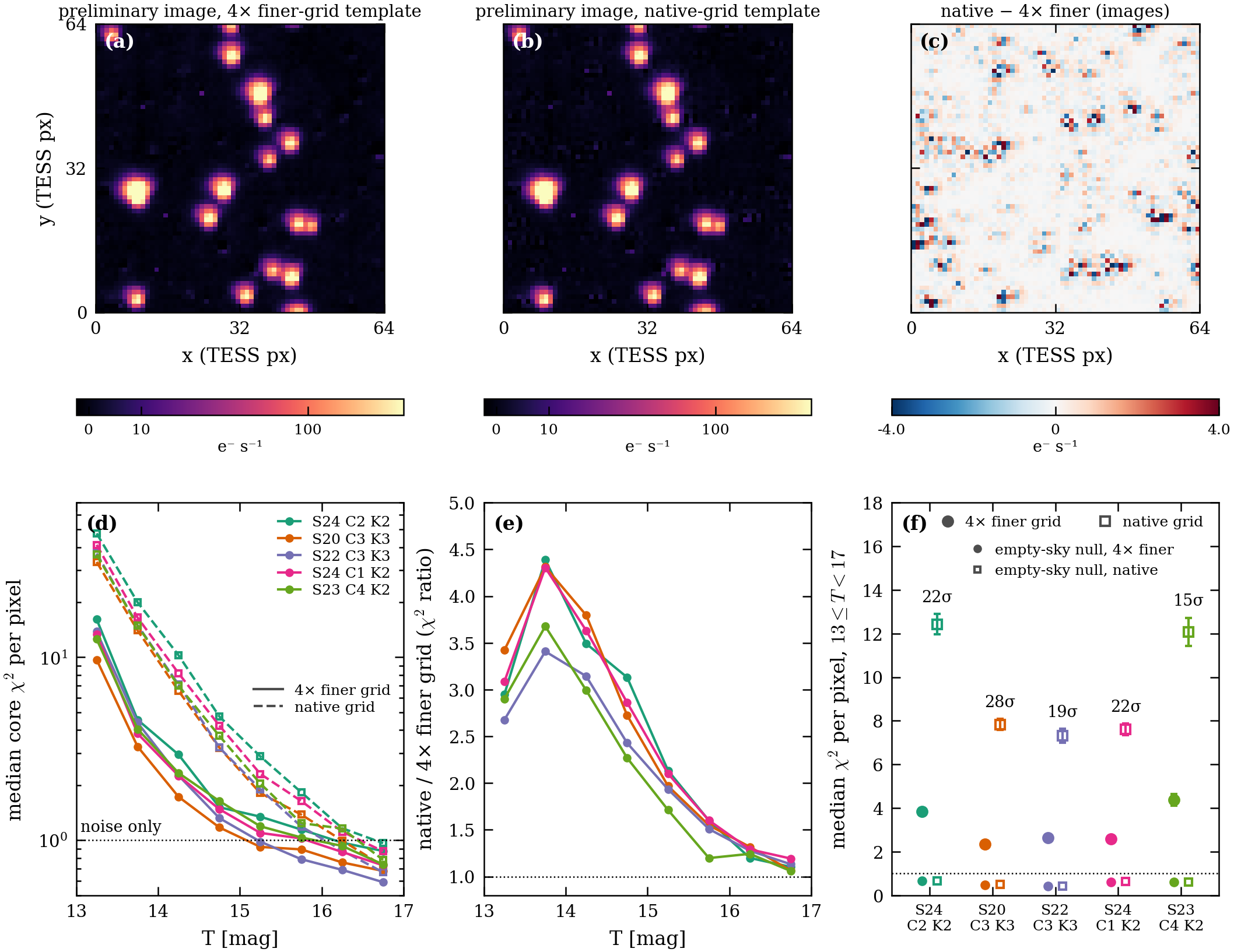
We compare the template built on the native TESS grid with one four times finer, on the same frame with the same settings. In the preliminary de-crowded image the native grid leaves a core $\chi^2$ 2.8–3.3 times larger at the stars that remain in the template (Fig. A1). The joint fit itself is much less sensitive: fitted to the native-grid preliminary image, the held-out core $\chi^2$ changes by a factor 0.97–1.07 at $T=8$–11, 1.02–1.12 at $T=11$–12 and 1.10–1.24 at $T=12$–13 (two folds in each of the five fields), so the finer grid matters mainly for the fainter stars.
Effect of the template sampling on the preliminary de-crowded image. (a, b) The same 64×64 TESS-pixel crowded box (S24 C2 K2) in the preliminary de-crowded image built with the 4× finer-grid template and with the native-grid template (identical asinh stretch), and (c) the difference of the two images, native − 4× finer. (d) Median core χ² per pixel (r ≤ 2.5 px) at the catalogue stars that remain in the template (13 ≤ T < 17), versus T, for the five fields (solid: 4× finer grid; dashed: native grid; dotted: noise only), and (e) the ratio native/4× finer. (f) Median χ² per pixel over all these stars: 3.85 → 12.43, 2.35 → 7.83, 2.63 → 7.32, 2.59 → 7.61 and 4.38 → 12.08 (4× finer → native; S24 C2 K2, S20 C3 K3, S22 C3 K3, S24 C1 K2, S23 C4 K2), i.e. a factor 2.8–3.3 (15–28σ), largest at T = 13–14.5; the empty-sky null (0.43–0.67) is unchanged and the red−blue residual dipole is unchanged within about 2σ (84–119 mpx; largest change S23 C4 K2, −8.7 mpx, 2.4σ). The empty-sky null is the robust variance $\chi^2_{\rm rob}=(1.4826\,\mathrm{MAD}(D/\sigma))^2$ of the residual $D$ in units of the noise estimate $\sigma$ over fixed empty-sky pixels; 0.43–0.67 means the noise estimate is conservative by 22–53 %, identically for both templates.
B Background details
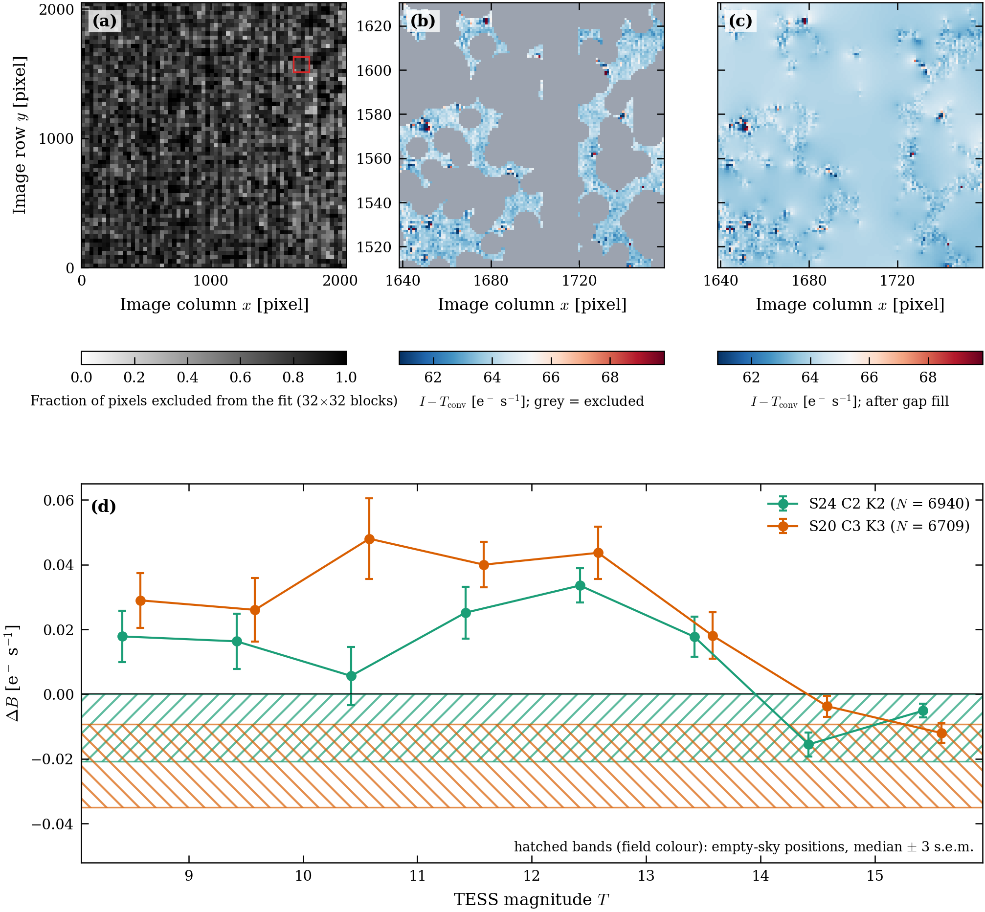
(a) Fraction of pixels excluded from the fit in 32×32 blocks (0.768 excluded overall): catalogue stars ($T<13$, magnitude-scaled disks), red $13\le T<16$ stars, saturated-bleed regions, two bad columns, and the standard mask. (b, c) $I-T_{\rm conv}$ over a 120×120-pixel region on the fit pixels, before and after harmonic gap filling. (d) Median background bias under isolated stars in 1-mag bins for S24 C2 K2 and S20 C3 K3, against empty-sky positions. Biases under stars are $\le0.05$ e$^-$ s$^{-1}$, below 0.1 % of the sky level.
C Band synthesis
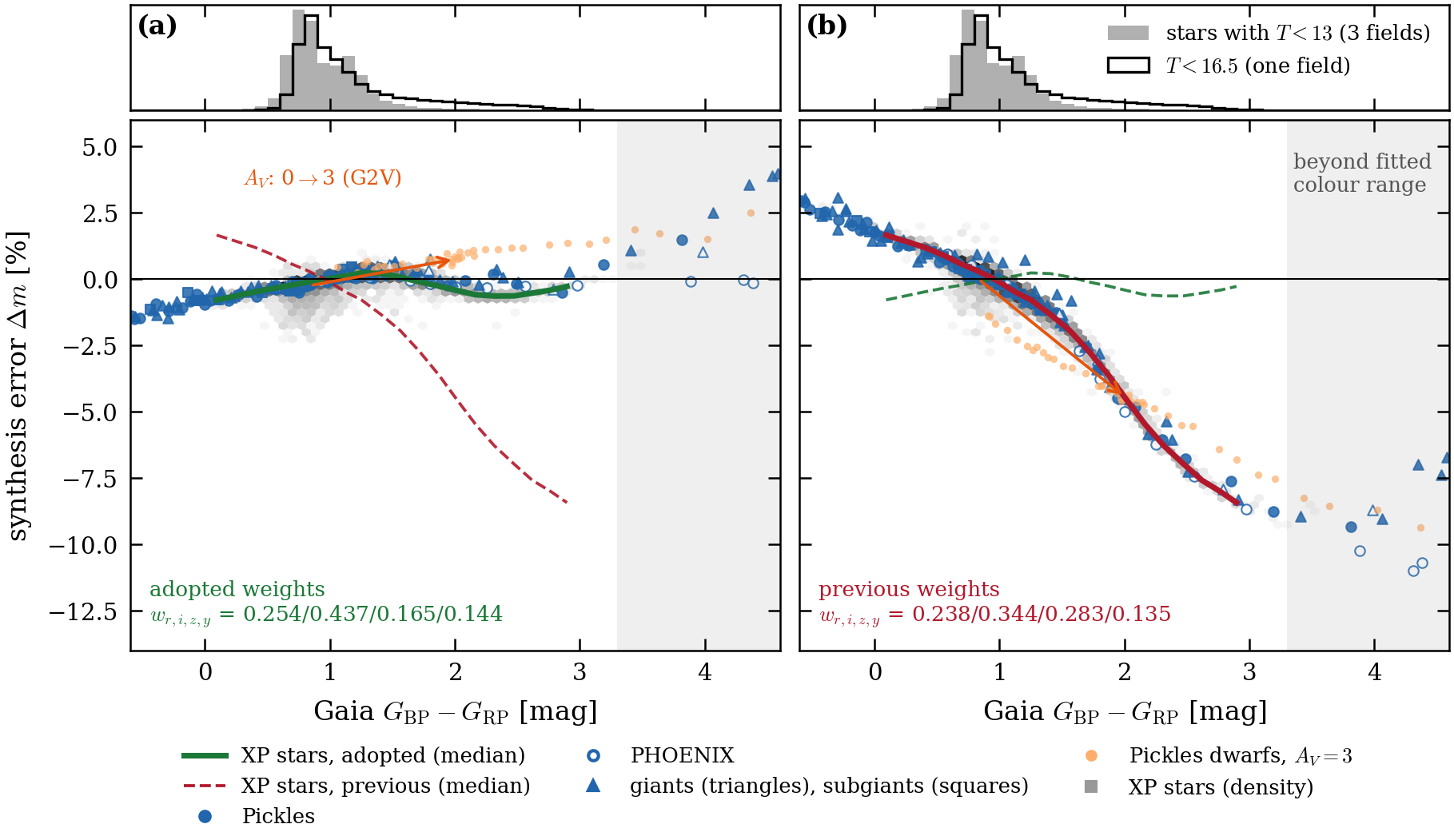
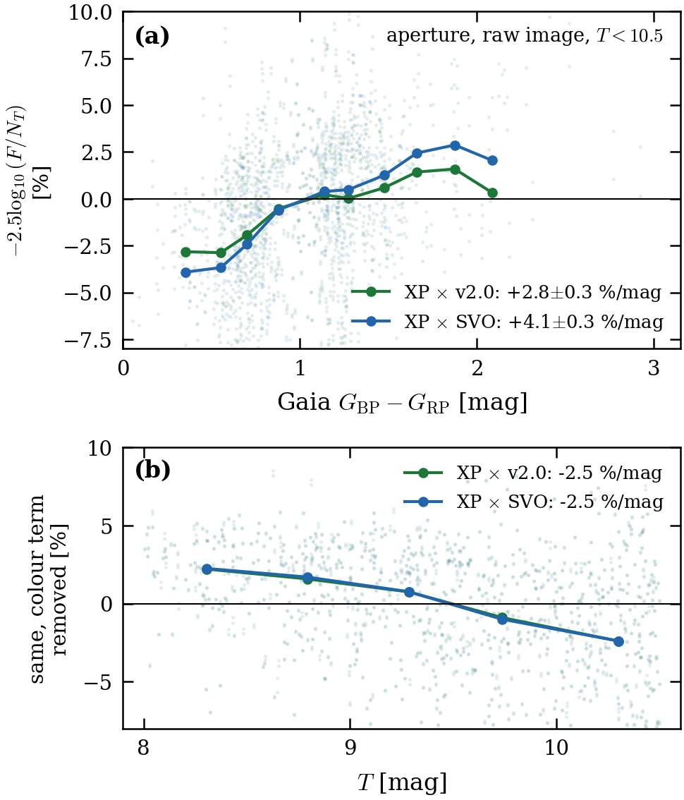
The weights of §2.2 are chosen so that the synthesised template follows the TESS count rate predicted from stellar spectra. Figure C1 shows the synthesis error against colour. Figure C2 shows the evidence for the TESS response curve used. In the model-free aperture fluxes of bright stars, version 2.0 of the TESS response leaves the smaller colour term: +2.8 against +4.1 % per mag for the SVO TESS.Red curve. Neither response gives a flat relation; the remainder is the red total-flux deficit of §6.
Synthesis error $\Delta m$ of the band mix against Gaia $G_{\rm BP}-G_{\rm RP}$ for model spectra and Gaia XP stars, for the adopted weights (a) and the previous weights (b). The previous weights are shown because the TESSreduce pipeline (Ridden-Harper et al. 2021) uses them. Shaded: colours beyond the fitted range. Histograms: the colour distribution of the stars.
Bright stars ($T<10.5$) of S24 C2 K2 in the raw image, 8-px aperture flux $F$ against the count rate $N_T$ predicted from Gaia XP spectra through TESS response version 2.0 (green) and the SVO TESS.Red curve (blue). (a) Against colour, with the slopes of a joint fit in colour and $T$ (the $T$ term removed). Points: stars; lines: binned medians. (b) The same with the colour term removed, against $T$. The $-2.5$ % per mag magnitude term has the sign of the bright-end flux-scale trend of §5.5 but is several times larger in this raw-aperture measurement; it is fitted jointly and does not change the colour slopes. Version 2.0 gives the smaller colour term; neither response is flat (§6). XP spectra are extended beyond 1020 nm with a power law.
| Spectral group | n | Previous weights | TESSreduce | Adopted weights |
|---|---|---|---|---|
| weights r,i,z,y | 0.238/0.344/0.283/0.135 | 0.256/0.276/0.358/0.112 | 0.254/0.437/0.165/0.144 | |
| O/B | 14 | +2.6 (+1.9…+3.1) | +2.7 (+2.0…+3.5) | -1.2 (-1.5…-0.8) |
| A | 18 | +1.7 (+1.3…+2.1) | +1.7 (+1.3…+2.2) | -0.7 (-1.1…-0.4) |
| F | 18 | +0.8 (+0.1…+1.1) | +0.8 (+0.1…+1.4) | -0.3 (-0.6…-0.1) |
| G/K | 43 | -0.3 (-1.6…+0.9) | -0.4 (-2.1…+1.2) | +0.1 (-0.5…+0.6) |
| K7–M3 | 24 | -3.6 (-6.8…-0.8) | -4.1 (-7.9…-0.5) | +0.1 (-0.3…+0.8) |
| M4–M6 | 10 | -8.5 (-10.2…-7.2) | -9.9 (-11.7…-8.4) | -0.1 (-0.5…+1.5) |
| late M (PHOENIX ≤2700 K) | 7 | -8.7 (-11.0…-6.7) | -9.3 (-12.5…-6.2) | +2.5 (-0.1…+4.0) |
D Colour models: physical operators against basis functions
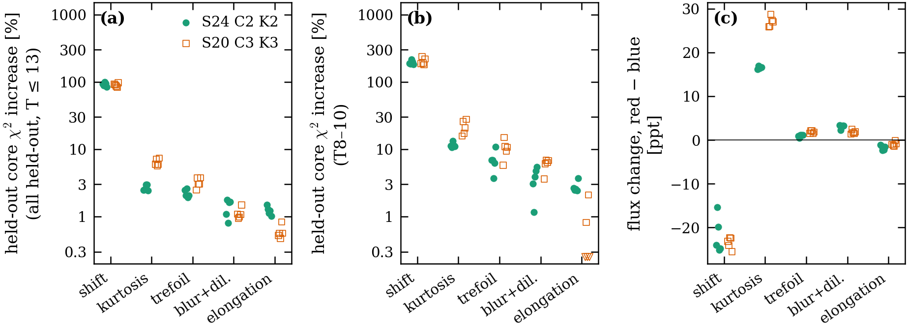
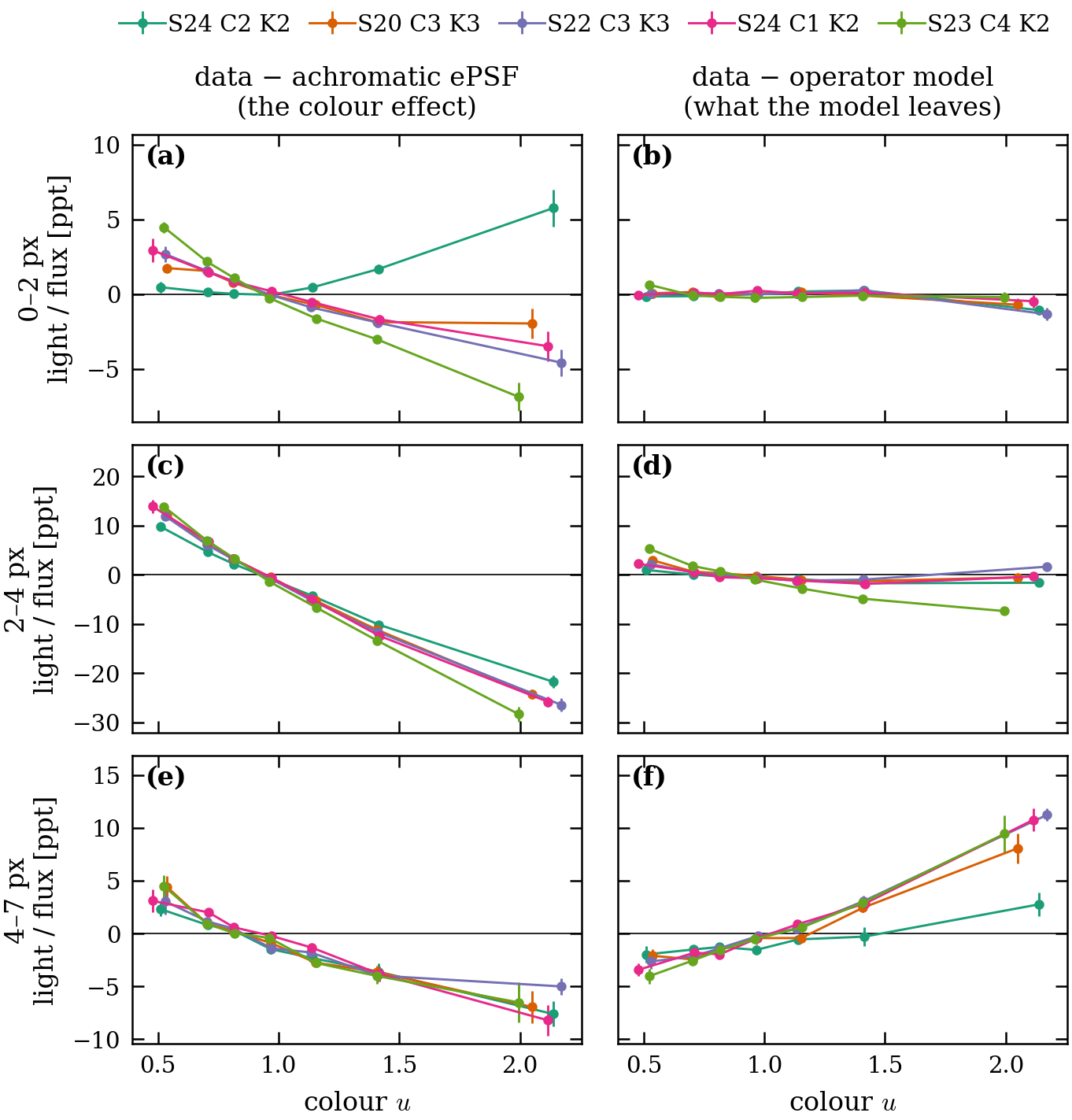
We first modelled the colour dependence with physical operators (lateral shift, kurtosis, blur and dilation, trefoil, elongation), each moving core and wing in a fixed ratio. Each operator lowers the held-out $\chi^2$ when added: the shift dominates, kurtosis follows, and the others cost 0.4–3.9 % when removed. The operators leave structure out to 3.5 px and over-remove far-wing light of red stars, because they change core and wing together. The basis-function model of §4.5 keeps the shift and replaces the other terms by ring and coma functions; its held-out $\chi^2$ is 0.91–0.96 of the operator model at $T=10$–13 and 0.68–0.88 at $T=8$–10 and for red stars (preliminary, two folds on three fields).
The operator model refitted on the preliminary image of two fields, once per fold, with one operator group held at zero and everything else unchanged; changes are relative to the full operator model on the same image and folds. (a) Increase of the median held-out core $\chi^2$, all held-out stars ($T\le13$); (b) the same at $T=8$–10; (c) change of the red ($u\ge1.3$) minus blue ($u<0.6$) median flux of held-out $T=10$–13 stars. Each point is one fold. Removing the lateral shift costs +83 to +99 % (+179 to +237 % at $T=8$–10) and biases the red minus blue flux by $-15$ to $-26$ ppt. Removing kurtosis costs +2.4 to +7.4 % (+11 to +28 % at $T=8$–10) and +16 to +29 ppt. Trefoil (+1.9 to +3.8 %), blur plus dilation (+0.8 to +1.8 %) and elongation (+0.5 to +1.5 %) each cost $\chi^2$ in every fold; at $T=8$–10 three S20 C3 K3 folds gain +0.2 % or less from elongation, one of them $-0.3$ % (open triangles at the lower edge). All 50 refits are shown.
Light in annuli of 0–2, 2–4 and 4–7 px around clean held-out $T=10$–13 stars, as a fraction of the star's flux (ppt), against colour $u$, five fields (median per colour bin with bootstrap errors; operator-model fits on the preliminary image, five folds per field). Left (a, c, e): data minus the achromatic ePSF, the colour effect itself. Right (b, d, f): data minus the operator model. Red stars have less light at 2–4 px ($-22$ to $-28$ ppt at $u\approx2.1$) and at 4–7 px than an achromatic PSF; S24 C2 K2 is the exception inside 2 px, where red stars have more light in the core. The operator model removes the colour effect to within 1.5 ppt inside 2 px (b) and within about 3 ppt at 2–4 px in four fields; on S23 C4 K2 it leaves $-7.4$ ppt for the reddest and $+5.3$ ppt for the bluest stars (d). At 4–7 px it leaves a red excess of up to +11 ppt (f): the model removes more far-wing light from red stars than the data lose, because each operator changes core and wing together in a fixed ratio. There is no red halo in the data (e).
E A linear peak-charge width term
We tested whether the effect of §4.6 can be absorbed by a brightness-dependent blur. For star $s$ the rendered PSF is $$P_s(x,y)=P(x,y)+\tfrac12\,\Delta\Sigma_s\left(\partial_x^2P+\partial_y^2P\right),\qquad \Delta\Sigma_s=b\,\frac{q_s}{10^{4}\,{\rm e^-}} ,$$ where $P$ is the fitted ePSF after the colour terms, $q_s$ the peak charge per 2-s read of §4.6 (computed once from the starting fluxes and held fixed) and $b$ one scalar per fit (px$^2$ per $10^4$ e$^-$), trained together with the ePSF, colour terms and WCS.
- The term removes about half of the observed broadening: the pooled slope falls from $(1.35\pm0.07)$ to $(0.76\pm0.07)\times10^{-3}$ px$^2$ per $10^4$ e$^-$, and the excess at $q>1.2\times10^4$ e$^-$ falls by 47 %. The trained $b$ is below the model-free slope in every field, and it is poorly pinned in a single image: in S22 C3 K3 it varies from 0.03 to $1.10\times10^{-3}$ between folds, and in tests on the fit to the final image the held-out $\chi^2$ was flat in $b$ between about 0.4 and $1.4\times10^{-3}$.
- Injected values of $b$ (0, 0.5 and $1.5\times10^{-3}$) in the real scene of a held-out fold are recovered without bias (to $\le0.012\times10^{-3}$; fit to the final image).
- The held-out $\chi^2$ per star falls by $4.6\pm0.8$ % at $T=8$–8.5 and, averaged over 0.5-mag bins, by $1.15\pm0.17$ % at $T=8$–10.5 and 0.12 % at $T=10.5$–13; it is unchanged at $T=9.5$–10.5. PSF magnitudes change by $-0.45$ mmag at $T\approx8.25$ and $+0.19$ mmag at $T\approx12.75$; on the fit to the final image, aperture fluxes within 3 and 5 px change by at most 0.35 ppt.
- A threshold in $q$ (zero below $3\times10^3$ e$^-$) brings the trained $b$ to the model-free slope and removes 66 % of the high-$q$ excess against 49 % for the linear form (fit to the final image, three fields, two folds); held-out $\chi^2$ does not prefer it. We did not pursue it further.
We also asked whether the broadening is better described as a Gaussian blur or as pixel-level charge transport (a brighter-fatter-like redistribution, built star by star at each star's pixel phase from the boundary flux $\tfrac12(I_i+I_j)(I_i-I_j)$ between neighbouring pixels $i,j$ of intensity $I$). Split into a $3\times3$ grid of CCD cells (Fig. E2), the bright-minus-faint stack is fitted equally well by both in every cell: $R^2$ 0.33–0.85 for the blur and 0.32–0.82 for transport, differing by at most 0.07, both leaving residuals of 0.9–1.4 times the noise, and fitting both together gains at most 0.02. With about 300 bright stars per cell the data cannot choose between the two mechanisms. Pooled per field, both smooth descriptions miss the central-pixel deficit of §4.6 ($-1.38\pm0.24\times10^{-4}$ px$^{-2}$, Fig. 14c).
We do not adopt the term: it captures only half of the effect; its single-image coefficient is poorly determined and differs between fields; the data cannot tell a blur from charge transport, and neither reproduces the central-pixel deficit; and it failed a pre-registered gate on the pooled median $\chi^2$ ratio ($0.9983\pm0.0004$ against the required 0.994; the median is set by the many stars at $T=9.5$–10.5, where the term has little effect). A complete model is future work.
(a) Excess width against peak charge, all fields pooled, without (grey) and with (red) the term. (b) Azimuthal profile of the $T=8$–9 minus $T=12$–13 stack difference, without and with the term. (c) Coefficient $b$ per field, trained (red), from all-star fits (blue) and the model-free slope of Fig. 14 (black). (d) Stacked residuals at $T=8$–9 without and with the term. (e) Ratio of held-out $\chi^2$ per star, with over without the term, per 0.5-mag bin.
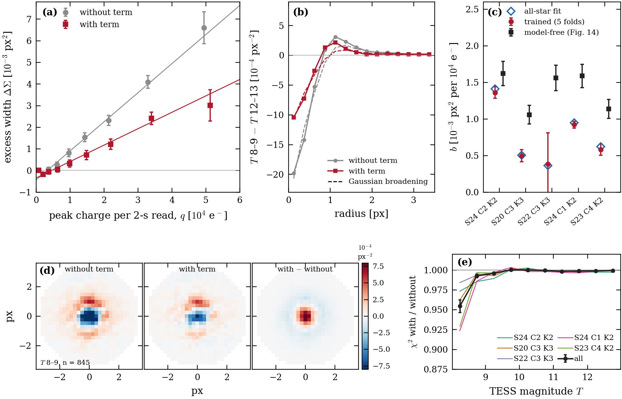
Bright-minus-faint residual stack ($T=8$–10 minus $T=12$–13, held-out stars of the fit to the preliminary image, five fields pooled) as an azimuthal profile in a $3\times3$ grid of CCD cells, oriented so that the optical axis lies beyond the top-left corner. Points: data with bootstrap errors. Red dashed: best-fit Gaussian blur; blue dotted: best-fit pixel-level charge transport; both fitted with flux, shift and constant terms. Each panel gives the number of bright stars, $R^2$ of both models and the residual rms in units of the noise. The two descriptions are indistinguishable in every cell.
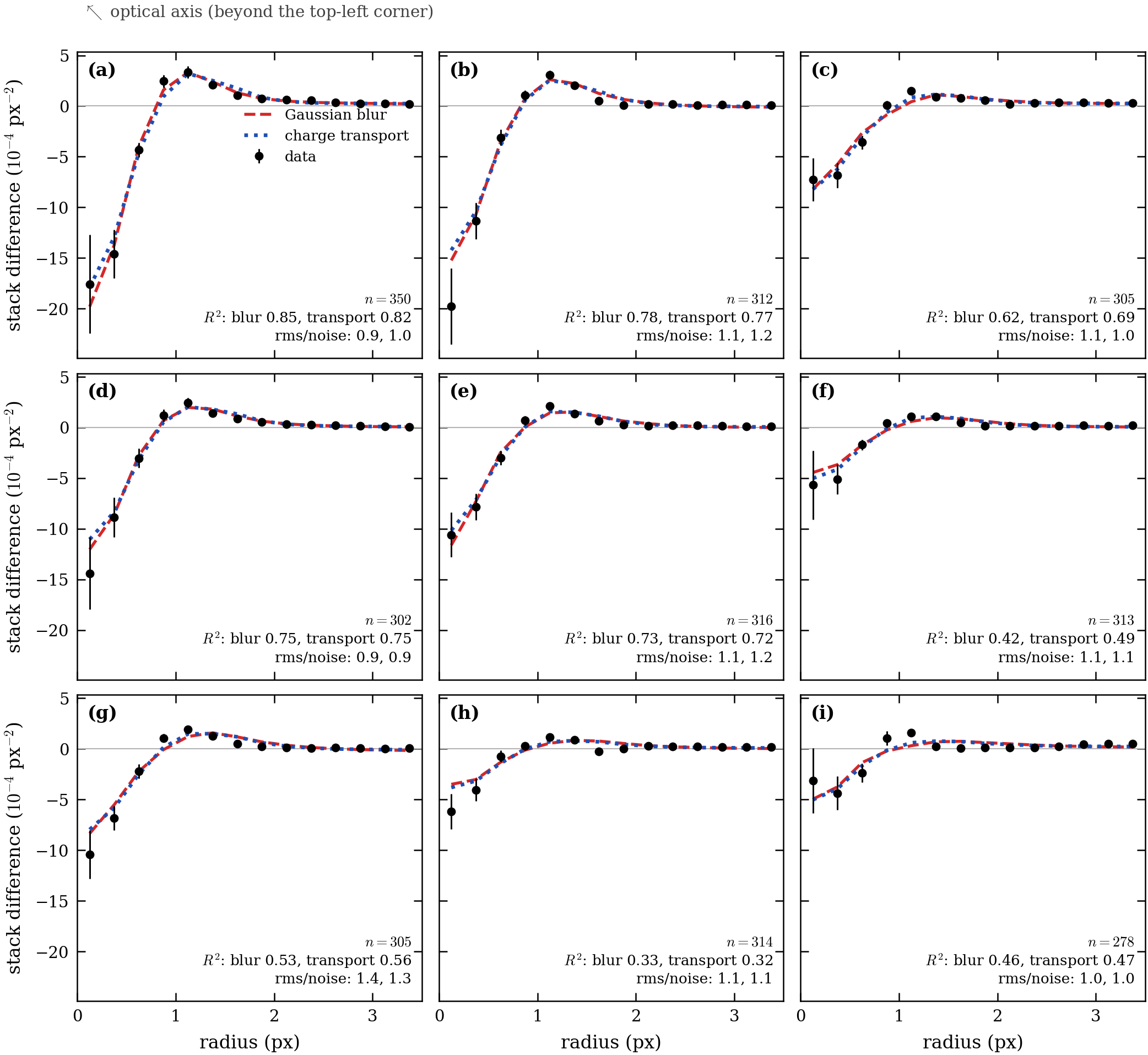
F Template core deficit near PS1 saturation
- Mid-colour stars just fainter than the bright-star removal limit show a 1.5–3 % positive core residual: the data are brighter than the template. It is gone by $T\approx14$, the same in two fields and with both Hotpants and the per-band kernels, so it is a property of the PS1 template, not of the subtraction.
- Stars saturated in at least one PS1 band persist to $T\approx13.9$, and stars within 0.5 mag of saturation to $T\approx14.2$, beyond the current removal limit of $T<13$. In $r$ the excess starts at the $r$ saturation line; in $z$ and $y$ it starts 0.5–1.5 mag fainter than their limits.
- Our measured onset is near $i\approx14.1$, with no excess at $i=14.1$–15. This implies a removal limit of $T<13.7$ (99 %) or $T<13.95$ (99.9 %). The pipeline is unchanged; this is a future-work line.
- Rest et al. (2014, §5.3.1) find deep stacks fainter than nightly stacks by $0.017\pm0.0013$ mag in $i$ for the brightest bin, "most likely the result of imperfect stacking algorithms of stars close to or at the saturation limit"; we cite this for the mechanism and sign only. Tonry et al. (2018) quote accurate photometry only for stars fainter than $m\sim14$; Chambers et al. (2016) note non-linearity from about 40,000 counts.
- A plausible reading, labelled as such: the seeing spread (peak proportional to flux over FWHM$^2$) moves the single-exposure limit of about 13.5 to about 14.1 in the stack, matching where our excess ends.
Core residual of stars with $0.8\le G_{\rm BP}-G_{\rm RP}<1.5$ against TESS magnitude and against PS1 $r,i,z,y$ magnitude, for Hotpants and for the per-band kernels, in two fields. Shaded regions and dashed lines mark the PS1 saturation levels. Both difference images show the same 1–3 % positive residual for $T\lesssim13.7$, which falls to zero about 0.5 mag fainter than saturation in $r$ and $i$.
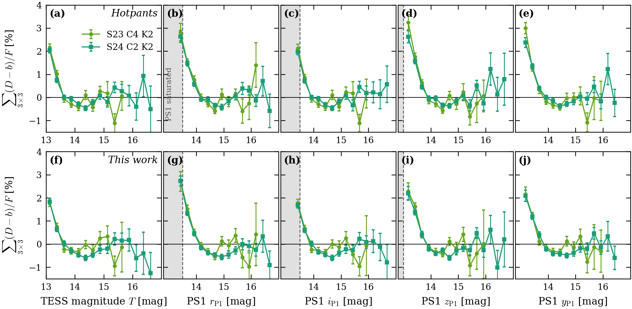
(a) Stars per 0.1 mag in S24 C2 K2, stacked by status: saturated in at least one band, within 0.5 mag of saturation, and farther. The dashed line marks the removal limit $T<13$. (b) Distance to saturation $\Delta=\min_b(m_b-m_{{\rm sat},b})$ for each star, coloured by $G_{\rm BP}-G_{\rm RP}$, where $m_b$ is the Gaia-XP synthetic PS1 magnitude and $m_{{\rm sat},b}$ the saturation level. Saturated stars reach $T\approx13.9$ and near-saturated stars $T\approx14.2$.